Ultra-high speed holographic shape and displacement measurements in the hearing sciences

The human ear is normally sectioned into three parts: the outer, middle, and inner ear, Fig. 1. The outer ear contains the auricle and external auditory canal. The middle ear is an air-filled space separated from the outer ear by the tympanic membrane (TM), or eardrum, with three ossicular bones (malleus, incus, and stapes) connecting the TM to the inner ear (cochlea). The cochlea is a fluid-filled structure that transduces acousto-mechanical motions into neural signals to the brain¹. During normal hearing, sound travels in the form of acoustic wave in the air and enters the external auditory ear canal to vibrate the TM². The vibration is then transmitted to the cochlea through the ossicles. Inside the cochlea, the sensory hair cells are set in motion to trigger nerve signals that are then received by the brain³.

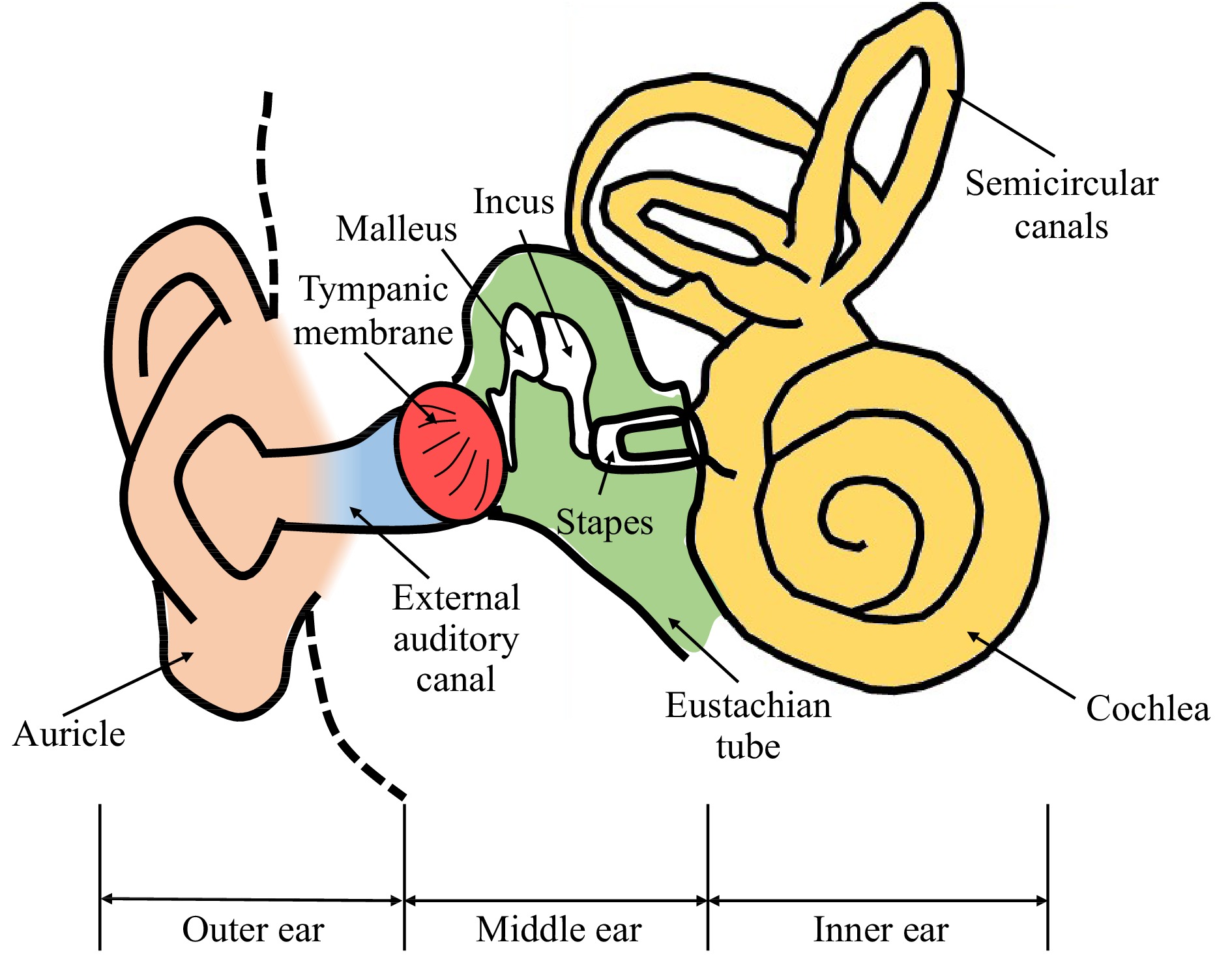
Fig. 1  Schematic of the outer ear, middle ear, and inner ear.

The thin semitransparent TM has unique anatomical and physical features that are critical to the hearing process^4,5. In particular, the adult human TM has an elliptical shape, measuring 9−10 mm horizontally and 8−9 mm vertically, with inhomogeneous, multi-layered, and anisotropic material characteristics⁶. It also has a flattened conical shape 2−3 mm in depth with apex directed inward towards the middle ear cavity. Characterization of the TM's morphology and vibration induced by acoustic excitation is essential to understand middle-ear structure and function in normal ears and in ears with pathologies such as otitis media with effusion, traumatic TM perforation, formation of retraction pocket and tympanosclerosis⁷⁻¹⁸.

We have been developing holographic methodologies utilizing ultra-high speed cameras up to 2.1 million frames per second^19,20 to quantitatively study the structure and function of the TM under different excitation conditions²¹⁻²⁷. As the frame rate of the camera is inversely related to the pixel density, in this study, we choose to run the camera at 67,200 frames per second to provide a field of view of the TM with a resolution of 512 pixels by 512 pixels. The 67,200 frames per second meets the Nyquist criterion for measuring the typical hearing frequency range from 20 Hz to 20 kHz^28,29. We have developed two high-speed techniques for TM shape measurements: the multi-wavelength technique³⁰ and the multi-angle technique³¹. The multi-wavelength technique uses a tunable laser source (to resolve optical phase differences to identify the shape) from a fixed angle of illumination³⁰; whereas the multi-angle technique uses a single wavelength laser source but with a dynamically changing angle of illumination (to introduce optical phase changes)³¹.

In this paper, we report our development of a new high-speed shape measurement approach that is based on fringe projection techniques to improve the optical efficiency and image quality during high-speed image acquisition for TM measurements. Also, because of the large amount of data that are collected during measurements, we report improved approaches to evaluate the optical phase. Our multi-wavelength and multi-angle techniques calculate the optical phase change during high-speed image acquisition using Pearson's correlation coefficient. Our previous coefficient calculations^30-33 included two levels of nested loops, which took a significant amount of the processing time. In this paper we report an optimized vectorized algorithm that removes the nested loops, greatly speeding up the Pearson's coefficient calculation.

This paper consists of introduction, results, discussion, methods and conclusion and future works sections. The physiology of the middle ear and the past developments of holography techniques on shape and vibration measurements for the middle ear research are discussed in the introduction section. The results section shows preliminary results of shape and vibration measurements of human TM, as well as National Institute of Standards and Technology (NIST) shape measurement comparison of the three shape measurement techniques. The methods section presents the principles of holographic vibration measurement utilizing Person phase correlation and shape measurement based on multi-angle and multi-wavelength configurations. Moreover, a miniaturized fringe projection is also discussed in the methods section and its schematics of the optical setups. The merits of different shape measurement techniques in applications for high-speed TM shape measurement are discussed in the discussion section. At last, the conclusion and future work are discussed.

The surface of a NIST traceable gauge was analyzed using high-speed fringe projection (HSFP) to demonstrate its working principle. A single fringe was projected and scanned across the sample’s surface by the scanning MEMS (Micro-ElectroMechanical System) mirror during image acquisition. Fig. 2 shows the experiment setup combining the HSFP with the high-speed digital holography (HDH) system. More details will be presented in the method section. Fig. 3a shows a single projected fringe. The single fringe images were grouped to form the four-step phase-shifted images based on the phase-shifting orders, as shown in Fig. 3b. Fig. 3b also shows multiple raw fringe images ($ {I}_{1}^{1},{I}_{1}^{2},{I}_{1}^{3},{I}_{1}^{4},\dots {I}_{q}^{m} $) at different MEMS mirror positions, where m is the phase-shifting order and q is the fringe order. Finally, the optical phase of the sample's shape, as shown in Fig. 3c, was obtained from the four reconstructed phase-shifted images.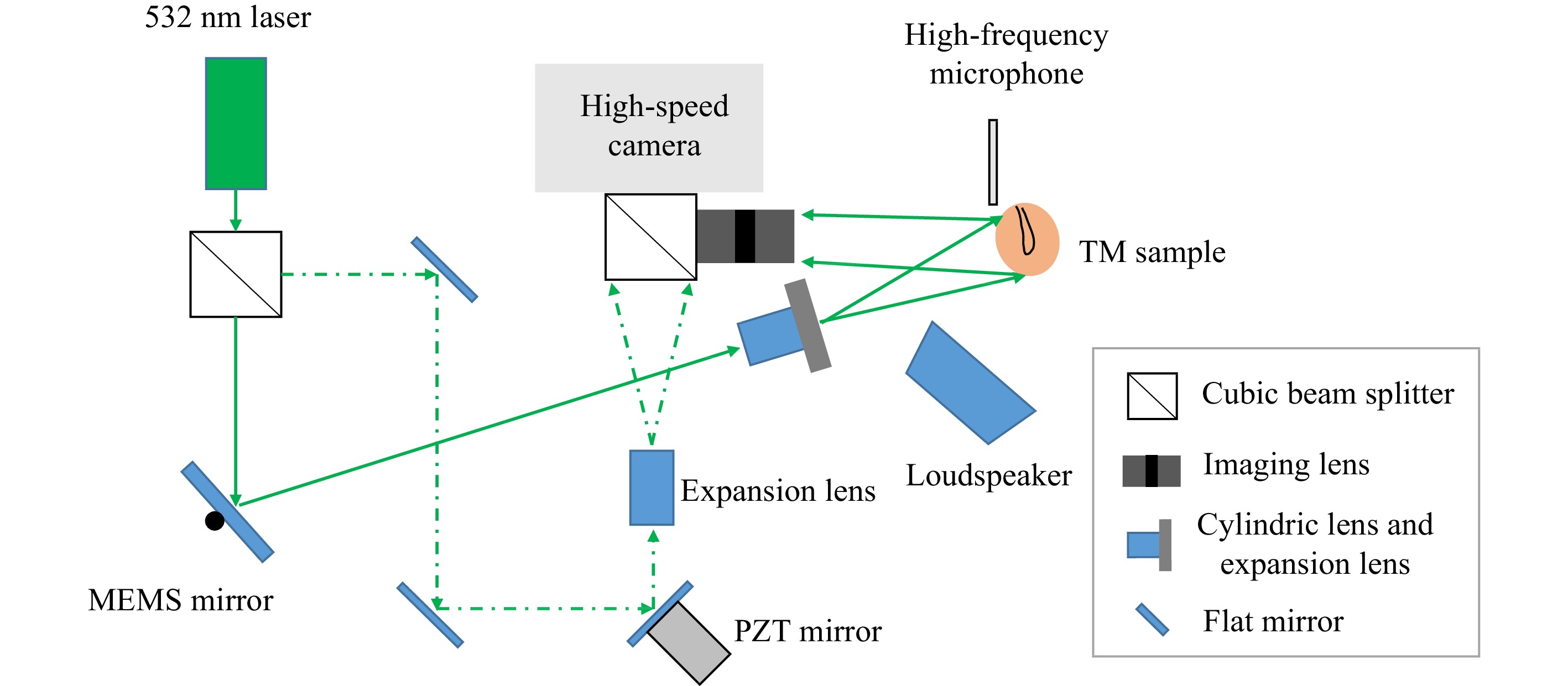

Fig. 2  Schematic of high-speed fringe projection and holographic displacement configuration. The MEMS mirror scans the sample's surface with a single fringe generated by the cylindrical and expansion lens for shape measurement. The PZT (piezoelectric ceramic material) mounted mirror is used to change the optical path for phase-shifting during displacement measurement. The middle ear sample is excited by transient click-like sounds produced by the loudspeaker. The sound wave near the surface of the TM is measured simultaneously by a calibrated broad range microphone.

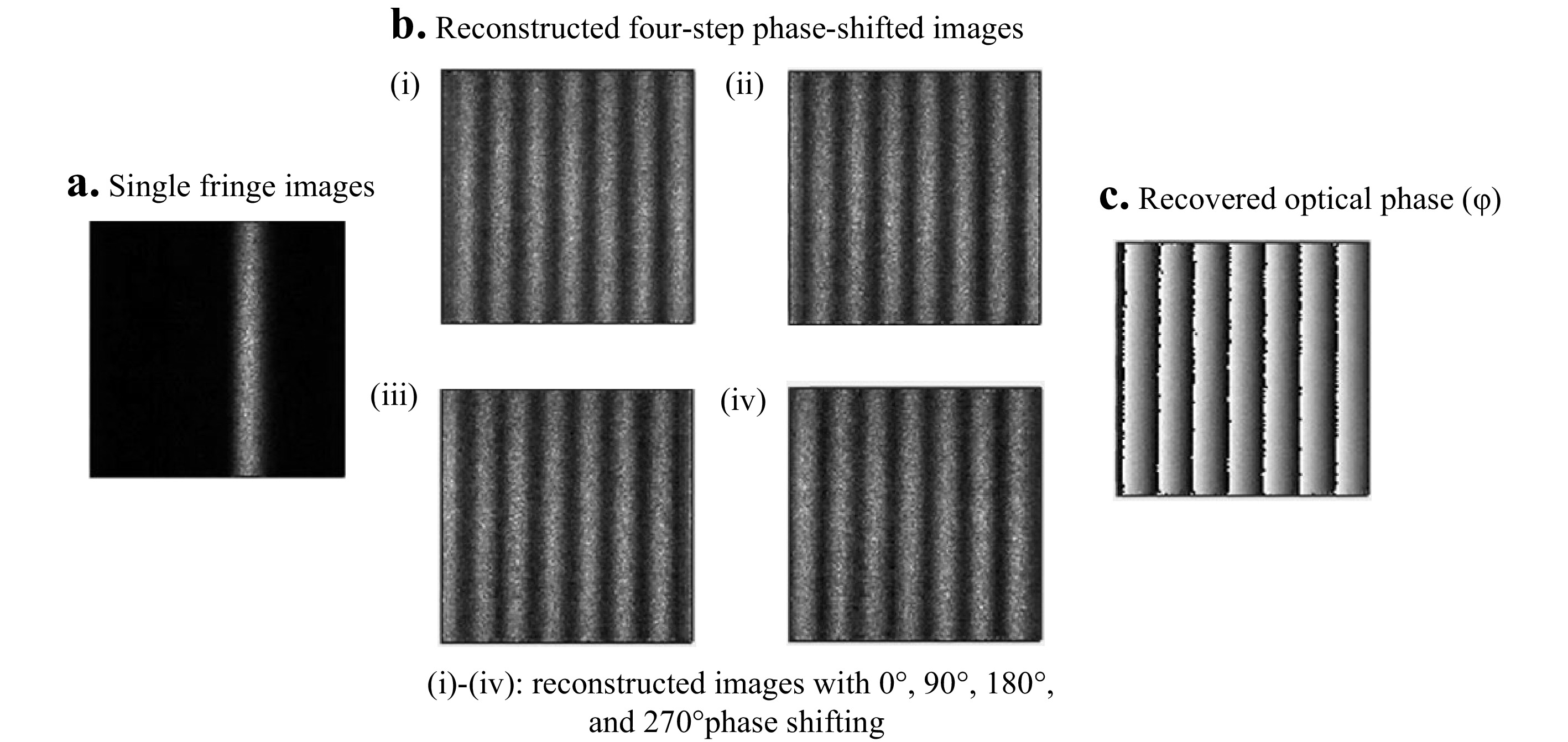
Fig. 3  Fringe projection measurement of a flat surface. a Raw single fringe images ($ {I}_{q}^{m} $) captured by a high-speed camera, where m indicates the phase-shifting order and q indicates the fringe order. b Reconstruction of four-step phase-shifted images; each multi-fringe image is the summation of $ {I}_{q}^{m} $ of the same phase order. c Optical phase of the flat surface obtained by the four-step phase-shifting method.

The dimensions of a NIST gauge are shown in Fig. 4a. The optical phase and 3D reconstructed shape measured by the Fringe Projection method is shown in Fig. 4b; Fig. 4c is the optical phase and 3d reconstructed shape measured by the multi-angle method. Fig. 4c depicts the optical phase and 3d reconstructed shape measured by the multi-wavelength method. In all 3D reconstructed shapes, the red line traces the height (in z-axis) of the middle section of the sample, where the lowest middle segment of NIST gauge is aligned to zero (z = 0). The average measured height profiles of the two end segments of the NIST gauge measured by three methods are 0.24 mm, 0.25 mm, 0.25 mm and 1.52 mm, 1.51 mm, 1.49 mm respectively. The standard deviations (σ) for the three segments are 0.042 mm, 0.037 mm, 0.014 mm; 0.053 mm, 0.023 mm, 0.014 mm; and 0.113 mm, 0.020 mm, 0.014 mm. The mean results agree with the dimensions provided by the manufacture of 0.25 mm and 1.50 mm, respectively, but for each position the standard deviations are smaller for the multi-wavelength method. The fringe-projection technique produced the largest σs.

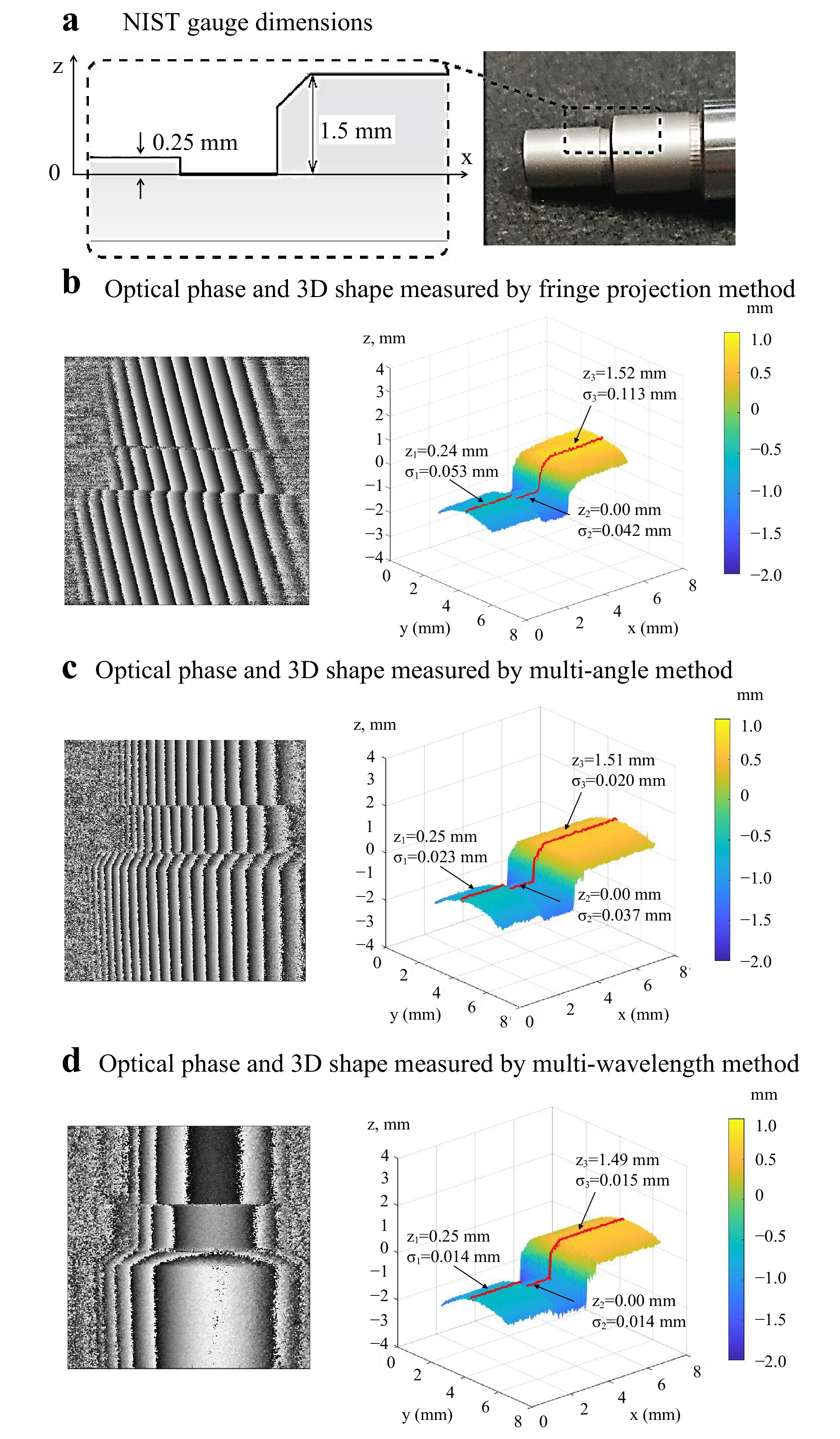
Fig. 4  Measurements of a NIST traceable gauge by three methods. a NIST gauge dimensions. b The reconstructed optical phase image and the 3D shape measurement result of NIST gauge by fringe projection method. c The optical phase and the 3D shape measurement of NIST gauge by the multi-angle method. d The optical phase and the 3D shape measurement result of NIST gauge by the multi-wavelength method. Z is the average height, and $ \text{σ} $ is the standard deviation of the given segment of each red line. All the $ {Z}_{2} $ are aligned to the zero position of the Z direction.

The three abovementioned shape measurement methods were used to measure the shape of one of three tympanic membranes (TM 1-3) from three cadaveric human temporal bones. Fig. 5 shows the three TM shapes measured using the HSFP, multi-angle, and multi-wavelength techniques, respectively. To assess variability within these measurement methods, a smoothing filter based on a moving kernel of 5x5 pixels size was applied and the standard deviation between the raw and the smoothed shape results were computed. Fig. 5a(i) shows the wrapped optical phase of TM1 obtained by the HSFP, and Fig. 5a(ii) depicts the smoothed 3D shape profile. The standard deviation between the raw and smoothed shapes obtained with HSFP is 0.11 mm, and the measurement was done by capturing 72 images in 25 ms. Fig. 5b(i, ii) shows the shape of TM2 measured by the multi-angle shape measurement method. The standard deviation is 0.15 mm, and the measurement was performed by capturing 1200 images in about 18 ms. Two pairs of four-phase-shifted images (total of 8 images) out of the 1200 images were chosen to reconstruct the shape at the optimal fringe density for phase unwrapping. Finally, Fig. 5c(i, ii) shows the shape measurement results of TM3 obtained with the multi-wavelength method, with a standard deviation of 0.13 mm. The measurement took about 150 ms due to the limitation of the wavelength tuning speed.

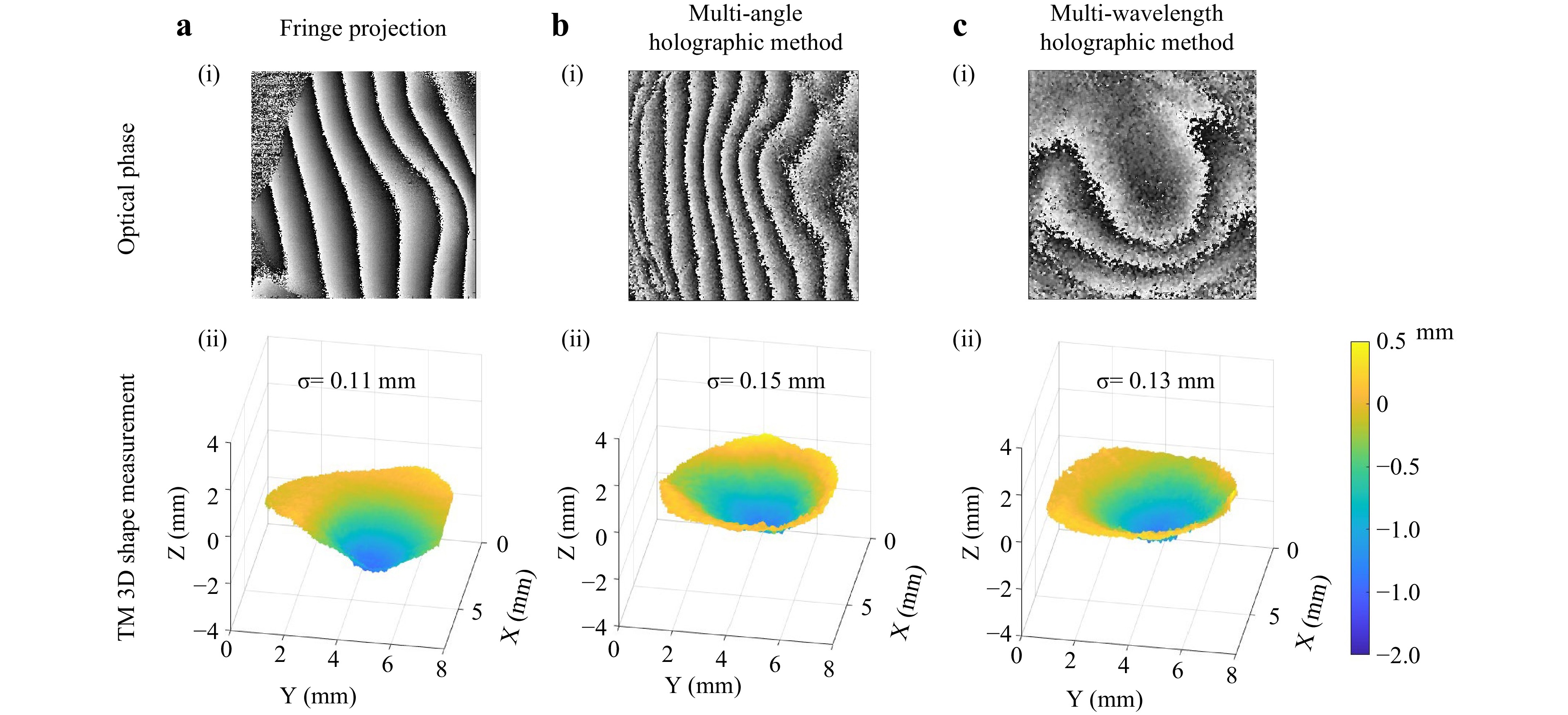
Fig. 5  Representative shape measurement results: Panel a is the shape result of TM1 measured by the high-speed fringe projection method, b is the TM2 shape measurement result by the multi-angle method, and panel c shows the shape measurement result of TM3 using the multi-wavelength method. The top panels (i) show optical phase maps and the bottom panels (ii) show 3D surface plots of the shape. The resolution in terms of standard deviation ($ \text{σ} $) for the three shape measurement results is 0.11, 0.15, and 0.13 mm, respectively.

To demonstrate the accuracy of the HDH displacement measurement, the surface displacements of a latex drum head of diameter 5 mm were measured with the HDH and compared with the displacement at the center of the drum (P1 in Fig.6) simultaneously obtained by an LDV (Polytec VFX-1-140). The latex drum head was excited using an impulsive sound generated from a loudspeaker. Fig. 6a shows a representative optical phase at 4.16 ms after the excitation. Fig. 6b compares the time-waveform of the displacement at P1 measured using the LDV and the HDH, showing a large overlap. The correlation between the two methods was found to be greater than 99%. Fig. 6c shows the Root–Mean–Square (RMS) pattern of the vibration from 3.5 ms to 7.5 ms after the excitation, with three markers: P1 is at the center of the drum where the LDV measures the displacement; P2 and P3 were chosen arbitrarily to show the lead and lag of the individual displacement on the sample's surface. Fig. 6d depicts the temporal evolution of the wavefronts of the three markers (P1 to P3) obtained using the HDH.

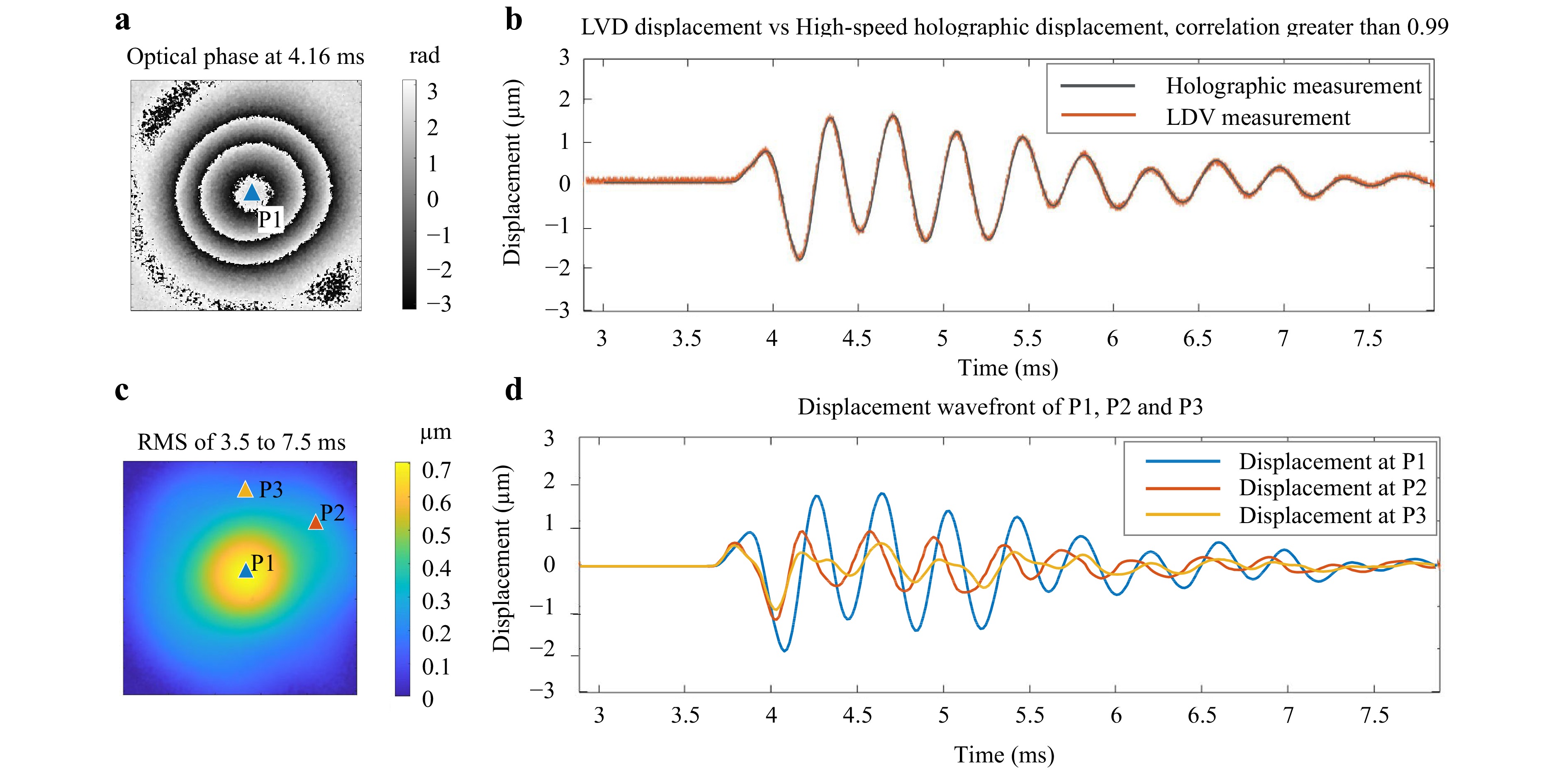
Fig. 6  High-speed displacement measurement results of a latex drum membrane and its comparison with the LDV result. The drum membrane is excited by a short acoustic click. The surface displacement of the membrane is captured by the high-speed holographic method, while the displacement of the center of the membrane is measured by an LDV. a The wrapped optical phase of the surface displacement at 4.16 ms after excitation. b Comparison of the displacement at the membrane center (P1 in c) measured by the LDV and the high-speed holographic method. c Root–Mean–Square (RMS) of the displacement 3.5 to 7.5 ms after excitation. The RMS is calculated based on the holographic displacement measurements along the temporal axis d Three individual displacement waveforms are marked in c from the holographic measurement results. The first 3 ms of the experiment is for the PZT phase shifter to scan the optical path to provide a 90-degree phase-shifted image, while the excitation starts at the 3.72 ms³⁰

Once validated, the HDH measured the displacements of a human cadaveric TM (TM1) induced by an acoustic click. The optical phase of the displacement was calculated using the vectorized Pearson's correlation coefficient algorithm to speed up the data processing. The vectorized algorithm's performance was compared with the previous nested-loop algorithm. Both algorithms generated the same optical phase shown in Fig. 7a. However, the vectorized algorithm took 0.17 s, whereas the nested loop algorithm took 3.54 s, using the same kernel size of 3 by 3 pixels (Fig. 7b). Clearly the vectorized algorithm outperformed the nested loop algorithm.

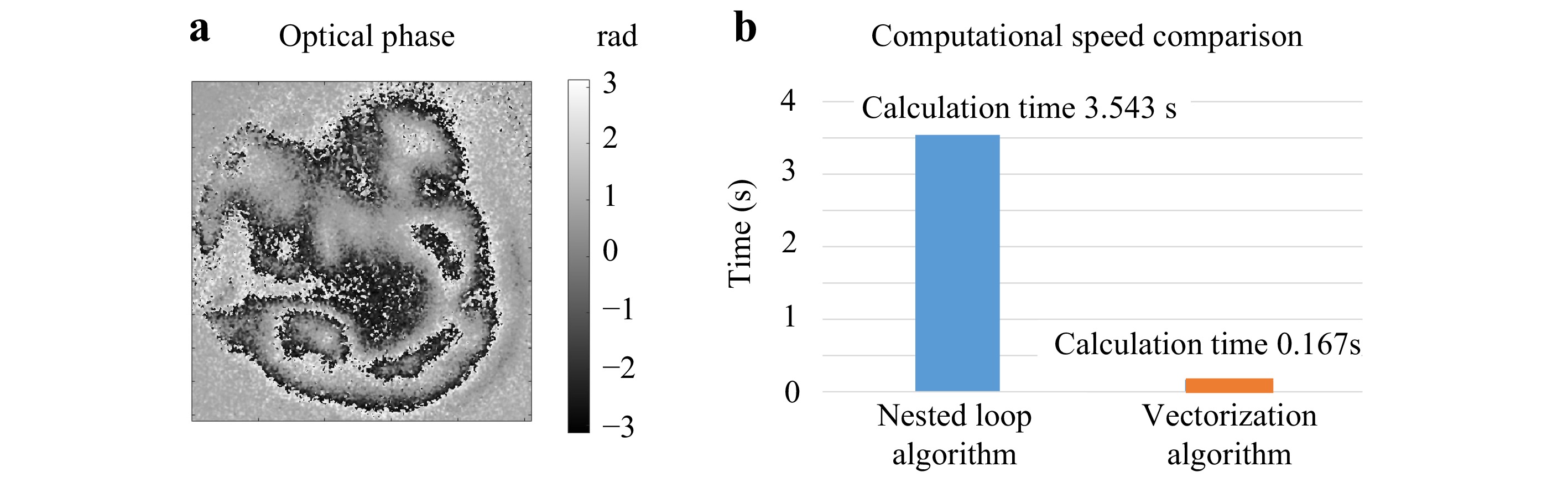
Fig. 7  Comparison of Pearson's correlation coefficient calculation of Optical Phase(OP) from a TM's High-Speed Displacement (HSD) measurement. a The OP of HSD measurement was obtained by the Nested Loop Algorithm (NLA) and the Vectorization Algorithm(VA). b the comparison of the computational speed shows the NLA takes 3.54 s and the VA takes 0.17 s to calculate the same OP.

A previous study demonstrated that the dominant displacement of the TM is perpendicular to its surface³². Therefore, the TM shape information was used to calculate the TM's surface normal vectors, which were combined with the holographic displacement measurements to determine the surface normal displacement. As a representative example, Fig. 8 shows the normal displacement component of a human TM sample when it was under an acoustic click excitation. Fig. 8a shows the 3D TM shape measurement results used to calculate the TM's surface normal vectors. Fig. 8b depicts the excitation signal, the click-like sound pressure near the TM produced by a loudspeaker. The RMS map of the surface normal displacement of the TM is shown in Fig. 8c. P0 is marked at the center of the ossicular attachment to the TM, and P1 to P4 mark the maximum RMS value in each quadrant. The individual wavefronts of P0 to P4 are shown at the top of Fig. 8d, while the bottom of the figure illustrates the magnitude of the computed frequency response at each location. These figures demonstrate that the amplitudes, cycles of vibrations, the leading and the lagging of the initial vibrations, and the time for each point to settle down are all different at different locations of the TM. The frequency and impulse responses computed from the stimulus and local displacements characterize location dependent TM mechanical properties and help differentiate various middle ear conditions corresponding to middle ear pathologies³⁴⁻³⁶.

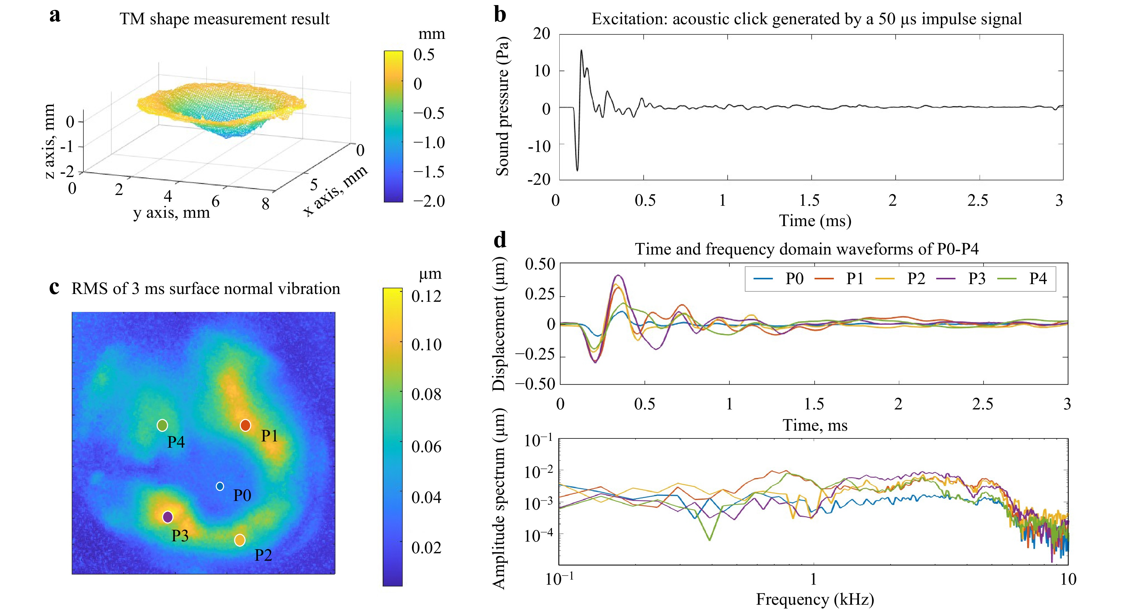
Fig. 8  High-speed holographic surface normal displacement results of a cadaveric TM. a The 3D shape measurement used in the calculation of surface normal vector. b The excitation signal to deform the TM is an acoustic click generated by a 50 µs impulse. c The RMS map of the first 3 ms of vibration normal to the TM surface after the excitation. The RMS is calculated based on the holographic displacement measurements along the temporal axis from 0 to 3 ms after the TM is excited by the acoustic wave. d Time-domain and frequency-domain wavefronts of the five individual points. The locations of these selected points are marked in c.

The discussion section compares the three-shape measurements based on their performance on a NIST gauge and applications on real TM samples, followed by discussion of the practicability of the three methods in TM measurements.

Table 1 compares the three shape measurement methods based on the results reported in this paper. The optical setup for the NIST gauge measurements was configured to mimic that used in the TM measurements, which met constraints like magnification requirements, the limited volume for triangulation, and available spatial resolution for the high-speed camera. The computed resolution is better (of lower value) in the NIST gauge measurements compared to the TM measurements because the NIST gauge is more reflective and does not need the higher illumination power required by the TM. Within the NIST gauge measurements, the resolution of the multi-wavelength method is better than the multi-angle, which is better than HSFP.

Performing high-speed imaging on semi-transparent samples such as TM requires a large illumination density, which significantly affects the optical phase quality of the results. The HSFP and multi-wavelength methods use the same 210 mW power laser light source, whereas the tunable laser output is 10 mW. Furthermore, the HSFP focuses all the available optical power on a single fringe, and can achieve the highest illumination power density of the three methods. In contrast, the multi-wavelength method has the lowest optical phase quality due to the tunable laser's lower illumination power. The image acquisition times for the fringe projection and multi-angle method are limited by the scanning speed of the MEMS mirror, and they have a similar measurement time of about 20−30 ms. The measurement time for the multi-wavelength method is limited by the wavelength tuning time of 150 ms. The processing time of the fringe projection method is much less than the multi-angle and multi-wavelength methods because the latter two need more computational power to track the four-step phase-shifted frames at each illumination position or wavelength.

The resolution of the shape measurement method is related to the optical phase quality as well as the sensitivity of the method's configuration. A comparison of factors that affect the sensitivity of the shape measurements is presented in Table 2. The sensitivity of the fringe projection method depends upon the projected fringe density and the triangulation of the illumination and observation direction. The sensitivity of the multi-angle method depends upon the illumination power as well as the illumination and observation direction and the angle difference of the illumination tuning. The multi-wavelength method's sensitivity depends upon the illumination and observation direction and the wavelength change. The fringe projection method has the highest resolution in terms of standard deviation among the TM measurement results and the lowest resolution among the NIST measurements. This may be because the fringe projection method can use the higher available illumination power when measuring the semi-transparent TM, whereas the additional power is not needed when measuring the NIST.

The HSFP method used in this paper is not compatible with temporal phase unwrapping, which requires a series of fringe images, where the fringe width gradually decreases to increase the fringe density. In HSFP the diameter of the laser beam determines the width of the fringe, and it cannot be changed automatically during the measurement in the current configuration. The multi-angle and multi-wavelength methods are suitable for temporal phase unwrapping since the spatial frequency of the optical phase of both methods changes gradually as the tuning of the illumination or the wavelength changes. By introducing temporal phase unwrapping, the resolution of the measurement results can be further improved³⁶.

The HSFP and multi-angle method require triangulation volume. Fringes projected perpendicular to the sample's surface are not sensitive to the shape of the sample along the projection direction. Thus, for both methods, there must be a triangulation volume to allow the scanning of the illumination. The human eardrum is located at the end of an approximately 2.5 centimeter long and 0.7 centimeter diameter ear canal, and the limited space favors the multi-wavelength method. However, the use of a higher power multi-wavelength laser would be advisable. For measurement of the cadaveric human eardrum, the ear canal can be removed to expose widely the TM, so we propose the multi-angle and fringe projection methods using the high-power fixed wavelength laser to measure the deformation and shape of the cadaveric human eardrum.

The HSFP applies a phase-stepping algorithm that utilizes four phase-stepped images. However, the maximum MEMS mirror's scanning speed is 3 kHz which is not fast enough to scan more than three fringes onto the sample during image acquisition by the high-speed camera since the longest exposure time of the camera is 0.001 s (1 kHz). Therefore, the system cannot capture the completed multi-fringe image in one frame. To overcome this limitation, the completed multi-fringe images are reconstructed after the image acquisition by summing up a series of single fringe images. The number of single fringe images needed is related to the width of the projected fringe and the desired fringe density. In this paper, a total of 72 images are captured to measure the shape of the human eardrum. The processing time of these images for a modern computer is less than 1 second allowing rapid examination of measurement quality.

The multi-angle method measures the shape of a sample by scanning the illumination across the sample. A PZT actuator is used as the phase shifter for the four-step phase-shifting algorithm. Locating the correct frames for the four-step phase-shifting method at each scanning position is done by scanning the Pearson correlation computed for each image to determine the shifted phase. This process for a total of 1200 images is more computationally expensive than the process of HSFP. Furthermore, with the multi-angle method, the illumination beam needs to be collimated and expanded to cover an area larger than the sample surface to maintain the illumination during the scanning and lowering the illumination density for high-speed imaging.

The multi-wavelength method utilizes a tunable laser for shape measurement. The wavelength is tuned during the high-speed image acquisition with a PZT actuator for phase shifting. A typical multi-wavelength shape measurement captures 50 high-speed images at 12 wavelengths. Within these 50 frames, four frames with 90-degree phase-shifted are selected via the calculation of the person correlation³⁷⁻⁴⁰ to calculate the optical phase at a given wavelength. Recording continuously while the phase shifter is moving linearly minimizes unwanted ringing within the phase shifter improving the accuracy of the phase shifting. It is possible to implement the method with 100 high-speed images at 12 wavelengths to improve the phase-shifting accuracy. The processing time of the multi-wavelength is similar to that of the multi-angle shape measurement. The output power and the tuning speed of the tunable laser limit the illumination power density and the measurement time. In our setup, the tunable laser only provides a minimal illumination power for the shape measurement, with a tuning time of 150 ms. A moving average filter has to be used to extract the optical phase due to the minimal illumination power reducing the spatial resolution of the shape measurement.

In summary, the multi-wavelength method does not require triangulation volume to measure the shape, but the optical power of these lasers are limited and the method generally requires painting of the TM. The Multi-angle method enables the shape measurement on the unpainted TM with more optical power, and the HSFP allows rapid shape measurement of the unpainted TM with the least post-processing time. However, both the Multi-angle and HSFP methods have constraints with the small triangulation volume. Therefore, the ideal approach to measure the TM through the intact ear canal in live ears will be to apply the Multi-wavelength method with a tunable laser with the desired optical power and tuning speed for high-speed imaging.

Digital holography (DH) can record and reconstruct an optical wavefield (amplitude and phase) by comparing the optical path difference of the reference and object beams captured by an optical sensor (camera). For a general holographic interference setup, the measured optical phase ϕ is given by the fringe locus function³⁶:

where d is the optical path difference vector and e is the sensitivity vector defined as³⁸

where λ is the wavelength of the laser, b is the observation unit vector, and s is the illumination unit vector. Generally, the object beam is reflected by a diffusive scattering object, and the measured optical phase contains high spatial varying speckle noise. Therefore, the optical path difference cannot be retrieved from a single optical wavefield. However, the change in the measured optical phase $ \left(\Delta \phi \right) $ from the two camera exposures is expressed as

where $ {{\boldsymbol{e}}}_{1} $ and $ {{\boldsymbol{e}}}_{2} $ are the sensitivity vectors at two camera exposures. The optical phase change $ \left(\Delta \phi \right) $ can be retrieved if the speckle distributions at the two exposures correlate with each other. Eq. 3 is the foundation of digital holographic shape and deformation measurement^36,37.

For shape measurement, assuming there is no object deformation during the measurement, the height information (shape) of the measured subject can be obtained by modulating either the magnitude or the direction of the sensitivity vector. The magnitude of the sensitivity vector can be changed by tuning the wavelength of the laser source, which is basically the multi-wavelength method. On the other hand, it is possible to modulate the direction of the sensitivity vector by altering the angle of the object beam, which is the multi-angle shape measurement method. The details about the experimental setups for high-speed multi-wavelength shape and multi-angle shape measurement methods can be found in our previous publications^{29,30,34−36} and are briefly described below.

Gauges traceable to the National Institute of Standards and Technology (NIST) were used to validate the shape measurement capabilities of the methods presented in this paper. We then applied these methods to measure the shape of human TMs and compare the measurement results obtained by the three methods, including illumination density, image acquisition speed, optical phase quality, resolution, processing time, temporal phase unwrapping compatibility, and the need for triangulation volume.

To verify the accuracy of the displacement measurement, a latex drum head subjected to an impulsive sound stimulus was simultaneously measured by the High-speed Digital Holographic system (HDH) and a Laser Doppler Vibrometer (LDV). The acoustically induced displacements of a human TM measured with HDH are presented in the results section to demonstrate the capability of the HDH system.

A tunable laser can be used to change the magnitude of the sensitivity vector by changing the wavelength of the laser source, as described in²⁹. The optical phase difference $ \left(\Delta \phi \right) $ of a holographic measurement of an object with two different wavelengths results in

In Eq. 4, the optical phase ($ \Delta \phi $) is the difference measured from the interference pattern captured by the camera. The wavelengths $ {\lambda }_{1} $ and $ {\lambda }_{2} $ are known experimental parameters for the tunable laser, and b and s are the observation and illumination vectors, respectively, which can be measured directly or obtained by calibration. The optical path difference vector d can be solved to extract shape information. In the simplified 2D case shown in Fig. 9a, P is a random point on the subject, B is the observation point, and S is the illumination point. In this case, the amplitude of the optical path difference vector d can be expressed as: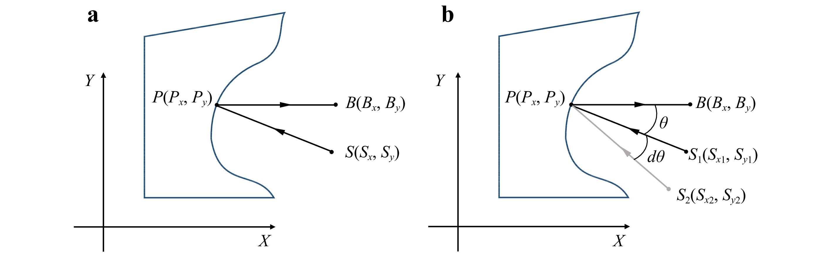

Fig. 9  2D Holographic schematic for shape measurements: a multi-wavelength experimental setup; b multi-angle wavelength experimental setup. The observation unit vectors are $ {\boldsymbol{P}}{\boldsymbol{B}} $ and the illumination vectors are $ {\boldsymbol{S}}{\boldsymbol{P}} $ for the two methods. $ {S}_{1} $ and $ {S}_{2} $ are the illumination points before and after changing the illumination angle in the multi-angle method.

where $ {P}_{y} $ is the user-defined pixel coordinates in the y-direction. $ {P}_{x} $, which contains the shape information in the x-direction, is the only unknown component of Equation (5) but can be solved for. Eqs. 4,5 show that as the wavelength change ($ {\lambda }_{1}-{\lambda }_{2} $) increases, the synthetic wavelength ($ {{\lambda }_{1}{\lambda }_{2}}/({{{\lambda }_{1}-\lambda }_{2}})) $ increases, and thus uncertainty of the shape measurement decreases.

The shape of the TM can also be measured by mechanically changing the direction of the illumination vector s. From Eq. 3,

where $ {{\boldsymbol{s}}}_{1} $ and $ {{\boldsymbol{s}}}_{2} $ are the illumination vectors at two camera exposures that can be measured or calibrated³⁰. The shape information is obtained by solving the optical phase difference using Eq. 6.

For the experimental arrangement shown in Fig. 9b, by introducing a known angle change (dθ) to the illumination vector, the height in the x direction can be determined by the following relation³⁶:

The sensitivity of the method increases as the angle change increases; moreover, it also depends on the non-zero illumination angle.

In this paper a third shape measurement method called fringe projection method was also implemented in our setup, which has several advantages comparing with the other two methods as being discussed in the Results and Discussion sections. A MEMS mirror (Brand: Mirrorcle) with a cylindrical lens was used to project a single fringe onto the sample, which was set up at its maximum scan rate of 3 kHz, and the frame rate and exposure time of the high-speed camera (Brand: Photron Fastcam SAZ, with a resolution of 512 by 512 pixels) were set at 67, 200 frames per second and ${1}/{67200} $ second, respectively. The camera was configured to be triggered by the position of the MEMS mirror to capture one image of a single fringe at each mirror position. All the single fringe images were summed up numerically to generate a synthesized, completed multi-fringe image after the high-speed acquisition.

The experimental setup for the high-speed fringe projection is previously shown in Fig. 2. The light source used is a 532-nm fixed wavelength laser (Oxxius). The laser beam is divided into a reference beam and an illumination beam. Two mirrors direct the reference beam to reach the expansion lens and are combined with the object beam at the beam splitter in front of the High-speed camera. The illumination beam first reaches the MEMS mirror, which has two rotation axes. The vertical axis rotation is used to switch the illumination to the cylindrical lens for fringe projection, and it is also used to switch the expansion lens for displacement measurements. The cylindrical lens is used to generate a single vertical fringe onto the sample. The horizontal rotation of the MEMS mirror is used to scan the single fringe across the surface of the sample during the shape measurement. The mechanical shutter in the reference beam is activated to block the reference beam for fringe projection during the shape measurement. The mechanical shutter is deactivated during the high-speed displacement measurement, and the MEMS mirror fixes the illumination beam to the expansion lens. The reflected light from the sample interferes with the reference beam on the beam splitter in front of the camera. Finally, the resultant speckle pattern is recorded.

The position of the fringes was based on the size of the sample and the configuration of the optical setup. The first single fringe image was taken at the left-most side of the field of view. The second MEMS mirror position was programmed to be at 90° phase-shifted position of the first fringe, the third at the 180° phase-shifted position, and the fourth at the 270° phase-shifted position. (Four-phase shifting was chosen for its balance of shifting speed and overall accuracy; however, any phase shifting strategy can be implemented.) This process was repeated until the entire sample was scanned. The repeatability of the MEMS mirror is examined by investigating the signal fringe image. The MEMS is programmed to project a signal fringe to a fixed position (Fig. 10a) for high-speed imaging and move the fringe out of the field of view back to its zero position. This procedure is repeated five times. A Gaussian curve is horizontally fit to the intensity image row by row, and the peak of the Gaussian profile is used to determine the position of the projected fringe. The difference in fringe position of the five consecutive measurements is 0.63 pixels, and the averaged fringe width is 100 pixels. The error introduced by the MEMS mirror in repositioning the fringe is less than 1% of the fringe width, and is assumed to be negligible.

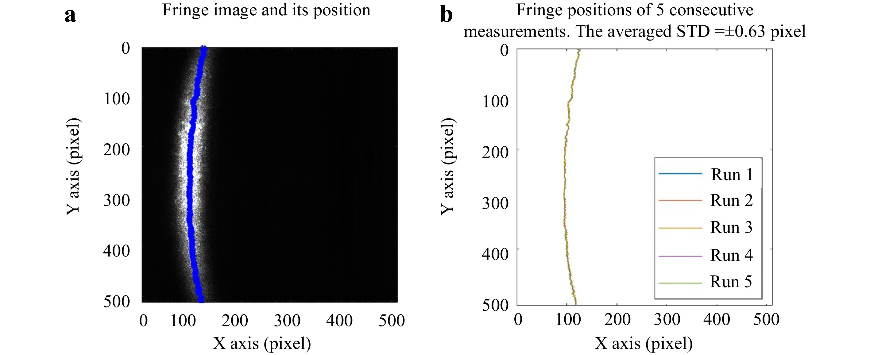
Fig. 10  The repeatability of the MEMS mirror is examined by checking the repeatability of the fringe position projected by the MEMS mirror during 5 consecutive TM measurements. a One fringe image with the Fringe position determined by averaged pixel position of the intensity image of each row. b the fringe position of 5 consecutive measurements and its averaged standard deviation is ± 0.63 pixels with averaged fringe width of 100 pixels. The reposition error introduced by the MEMS mirror is less the 1% of the fringe width and is assumed to be negligible.

Once all the single fringe images were captured, they were divided into four groups based on the angles of phase-shifting (0°, 90°, 180°, and 270°). The phase-shifting is calibrated based on the optical setup by making the distance between each projected fringe to be $ {W}/{4} $, where W is the width of the single fringe. The four-step phase-shifted multi-fringe images represented the numerical summation of each image group. The optical phase of the shape of the sample was calculated using Eq. 8.

The fringe projection shape measurement method is based on the projection of well-defined fringe patterns onto the sample. In the high-speed fringe configuration, the high-speed camera captures the 4n single fringe images sequentially, $ {I}_{1}^{1},{I}_{1}^{2},{I}_{1}^{3},{I}_{1}^{4},{I}_{2}^{1},{I}_{2}^{2},{I}_{2}^{3},{I}_{2}^{4}\dots {I}_{n}^{1},{I}_{n}^{2},{I}_{n}^{3},{I}_{n}^{4} $, where the superscript indicates the phase-shifting order and the subscript indicates the fringe order. Numerical summations $ ({I}_{1}^{1}+{I}_{2}^{1}\dots {I}_{n}^{1}) $, $ \left({I}_{1}^{2}+{I}_{2}^{2}\dots {I}_{n}^{2}\right) $, $ ({I}_{1}^{3}+{I}_{2}^{3}\dots {I}_{n}^{3}) $, and $ \left({I}_{1}^{4}+{I}_{2}^{4}\dots {I}_{n}^{4}\right) $ are calculated to reconstruct the completed multi-fringe images corresponding to the four-step phase-shifting frames. The optical phase φ of the shape of the sample is³⁷

The displacement measurement method measures the full-field-of-view (> 200,000 points at 67,200 camera frame rate) transient displacements^{29,31,32−35}. The Pearson's correlation coefficients between the deformed frame and two undeformed reference frames with 0 and 90° phase-shifting are calculated to quantify the optical phase of the sample's displacement. Assuming $ {I}_{r} $ is the intensity of the reference beam and $ {I}_{o} $ is the intensity of the object beam, and φ is the optical phase difference between the object and the reference beams. The interference patterns of the reference (undeformed) $ {I}_{ref} $ and deformed $ {I}_{def} $ states can be expressed as shown in Eqs. 9,10^29,38, respectively:

where $ \Delta \phi $ is the optical phase change due to the sample's deformation. To extract $ \Delta \phi $, we calculate the Pearson's correlation coefficient of a small window (e.g., 3 by 3 pixels) between the deformed and reference frames by using Eq. 11⁴⁰

where operator <> presents the expected value. Since the speckle pattern captured by the camera sensor is randomly distributed and the two same-sized matrices can be correlated, the expected value of the speckle pattern is equivalent to its numerical average³⁹. Assume φ is uniformly distributed and $ \Delta \phi $ is constant within the small window, then the coefficient can be simplified in the following format by inserting (9) and (10) into (11)³²:

where $ r={{I}_{o}}/{{I}_{r}} $ is the intensity ratio of the object and reference beams. Therefore, the optical phase difference due to the deformation of the sample can be calculated by²⁹

where $ \left({I}_{ref+\frac{\pi }{2}}\right) $ is the 90° phase-shifted reference frame of the undeformed frame. Khaleghi et al. have demonstrated that the dominant deformation of the TM is along the surface normal direction⁴⁰. Razavi⁴⁰ demonstrated that the sensitivity vector of the holographic system varies when the sample is located close to the imaging lens; however, the magnitude of displacement (S) along the surface normal direction, can be compensated by the sensitivity vector variation K(x,y) and the surface normal vector of the sample n(x,y), can be measured as $ \Delta \phi (x,y,t) $³⁴

where x and y are the pixel coordinates of the camera and t is the time.

Pearson’s correlation coefficient was used to calculate the optical phase between two camera exposures. The previous algorithm used a sliding window technique on each recorded image. The process consists simply of moving a sliding window (e.g., 3 by 3 pixels) from point to point in the horizontal and vertical directions. Calculating the Pearson’s coefficient of two of 512 by 512-pixel images requires more than 250,000 iterations, which takes about 3.5 seconds on a modern computer. For a typical displacement measurement, more than 1000 images are captured, which takes about one hour to finish the process. The long processing time makes accessing the measurement quality during the measurement impractical. The algorithm is optimized by a vectorization procedure to remove the nested loops to improve the computational performance. Vectorization is the process of converting an algorithm from operating on a single value at a time to operate on a set of vectors or matrices at one time utilizing the vector operation capabilities of modern CPUs.

To generalize the Pearson's correlation coefficient calculation for n by n kernel size (n=3,5,7…), defining $ {I}^{\text{'}}(i,j) $ are $ {n}^{2} $ translated matrices of the original image matrix I, where i= 1,2,3…n and j = 1,2,3…n. and $ {I}_{x,y} $ is the matrix element at (x,y) coordinate, $ {I}^{\text{'}}\left(i,j\right) $ is obtained by translating $ {I}_{x,y} $ by the following Equation:

Both the undeformed frame $ {I}_{ref} $ and deformed frame $ {I}_{def} $ are translated to $ {{I}_{ref}}^{\text{'}}\left(i,j\right) $ and $ {{I}_{def}}^{\text{'}}\left(i,j\right) $ by Eq. 15. The Pearson's correlation coefficient of $ {I}_{ref} $ and $ {I}_{def} $ can be calculated by Eq.11, and simplified expression is:

where $ X={{I}_{ref}^{\text{'}}}\left(i,j\right)-\frac{1}{{n}^{2}}\sum _{i}^{n}\sum _{j}^{n}{[{I}_{ref}^{\text{'}}}\left(i,j\right)]\;{\rm{and}}\;Y={{I}_{def}^{\text{'}}}\left(i,j\right)- $$ \frac{1}{{n}^{2}}\sum _{i}^{n}\sum _{j}^{n}{[{I}_{def}^{\text{'}}}\left(i,j\right)] $. The fastest calculation is the 3 by 3 pixels kernel version because it requires the minimum number of translated matrices, which takes about 0.15 s to finish on a modern computer. This 3 by 3 pixel kernel of the Pearson’s coefficient is suitable for displaying the results immediately after the measurement to assess the optical phase quality to determine if the measurement needs to be repeated.

The high-speed holographic displacement measurement method described in this paper utilizes the optimized Pearson's correlation algorithm to calculate the optical phase change introduced by the surface deformation of the sample. With the optimized algorithm, the calculation becomes 21 times faster using the same computation power. The improved processing speed makes it possible to display the optical phase of the high-speed image immediately after the acquisition for us to examine the measurement quality between the measurements, which streamlines the experiment process and makes measurements on live ears more practicable.

This paper presents a newly developed shape measurement method using a miniaturized fringe projection system with a Microelectromechanical systems (MEMS) mirror. We compared this method to measure the shapes of a NIST target and human TMs with two previously developed methods: (1) multi-wavelength method and (2) multi-angle of illumination method. We also present vibration measurements of human TMs made with an upgraded holographic displacement system, which is validated by comparing the holographic results of a vibrating drum head to simultaneously measured LDV results. For the shape measurement, the multi-wavelength method performs best on measuring the NIST target, while the measurement quality decreases on measuring the human TM due to the lower power of the tunable laser. The fringe projection and multi-angle methods can measure the unpainted TM due to the adaptation of a higher power laser. The fringe projection method requires fewer captured images than the multi-angle methods, making it a more practical shape measurement for live animal study. However, the fringe projection method and multi-angle method require triangulation volume, posing challenges to measurements made through an intact ear canal.

In the future, we will continue developing the displacement and shape measurement in the direction of utilizing the multi-wavelength method by identifying a suitable high power tunable laser for this application. The future implementation will be combined with the HSH system with an endoscopic configuration to allow measurements of the eardrum shape and responses through the intact ear canal in live ears. We have experimented with the Dynamic Time wrap algorithms to integrate the time series data for displacement pattern extraction from the holographic measurements. We will apply more artificial intelligence and data mining technologies to automate and streamline the data process.

Grant support from the US National Institute on Deafness and Other Communication Disorders (NIDCD R01 DC016079) is gratefully acknowledged. We would also like to acknowledge partial support by the Center for Holographic Studies and Laser micro-mechaTronics (CHSLT) at WPI. We also thank all of the reviewers of this manuscript for their insightful suggestions and input.