Measurement techniques for aspheric surface parameters

Asphere is a general term for surfaces that deviate from a sphere^1-3. The phrase ‘aspheric surface’ used herein is specific to a rotationally symmetric aspheric surface. Compared with a spherical surface, which exhibits the same curvature, an aspheric surface exhibits different curvature. Aspheric surfaces have higher degrees of freedom than spherical surfaces, thus allowing them to perform more functions. For example, aspheric surfaces can correct high-order aberrations and improve imaging quality, thus enabling effects that are only possible using multiple spherical mirrors and reducing the size of the optical system. Consequently, optical designers are inclined to use aspheric surfaces in modern optical systems, such as biomedical, lithographic, astronomical optics, and high-power laser systems, when considering system volume and imaging quality^4-9. The design and manufacturing capabilities of aspheric surfaces have gradually improved and high-order aspheric surfaces have become increasingly well-known owing to the increasing demand for aberration correction in optical systems^10-14. Sloan et al.¹¹ designed a double-Gaussian system and used three eighth-order aspheric surfaces to improve the image quality of an optical system. Yatsu et al.¹² reduced the zoom lens length of a camera by 30% using only a 10th-order aspheric surface instead of spherical surfaces. Optical systems with aspheric surfaces are continuously being improved owing to the ongoing development of optical design theory^15-26. The use of aspheric surfaces, particularly high-order surfaces, in optical systems is expected to increase.

The measurement of aspheric surfaces is vital to their manufacture. Although fabrication technology has developed rapidly in recent years^27-35, advances in fabrication technology have occasionally exceeded measurement capabilities. A well-established corollary of the saying, ‘you cannot make it if you cannot measure it’ has been established recently, i.e. ‘If you can measure it, you can indeed make it’. Manufacturing process bottlenecks typically arise from a lack of routine, cost-effective, and timely metrology solutions³⁶.

An aspheric surface is primarily measured based on its form and parameters. The surface form is the three-dimensional distribution of the surface in the spatial domain. The measurement result of the surface form is a geometric quantity that is typically expressed in terms of the surface height, which is a function of the (x, y) coordinates in units of length. Meanwhile, the aspheric surface parameters (ASPs) are well-defined quantities that can be derived from the surface form. Measurements of the surface form and parameters can be used to assess the aspheric surface quality. According to the international standard ISO 10110-12³⁷, the general expression for a rotationally symmetric aspheric surface comprises a conic term and an even term for the power series. The surface form is expressed as shown in Eq. 1.

In Eq. 1, R, K, and A_2i are the ASPs; R is the vertex radius of curvature; K is the conic constant; A_2i is the high-order aspheric coefficient; h is the surface height perpendicular to the z-direction; and z is the sag of the aspheric surfaces. Fig. 1a shows a schematic illustration of the change in the quadratic aspheric surface with respect to R when K = 0.6. Fig. 1b shows a schematic diagram of the change in the quadratic aspheric surface with respect to K when R = 40. Fig. 1c shows a schematic illustration of the addition of the fourth-order coefficient A₄ to the aspheric surface based on the quadratic aspheric surface. The length units of the vertical and horizontal axes in Fig. 1 are in millimetres, and the different line types and colours correspond to the various ASPs. Fig. 1 shows that R directly affects the overall curvature of the aspheric surface, the focal length of the aspheric surface, and the curvature near the vertex. Meanwhile, K determines the surface characteristics and type of aspheric surface¹⁰. Table 1 shows that K determines whether an aspheric surface is ellipsoid, spherical, paraboloid, or hyperbolic when it is quadratic. K exerts a minimal effect on the curvature near the vertex. The high-order aspheric coefficient A_2i is a high-order term added to the quadratic aspheric surface to further adjust the aspheric surface form, which barely affects the curvature near the vertex but significantly affects the curvature at the edges. The aforementioned parameters typically characterise an aspheric surface and are used in the entire design, fabrication, testing, and adjustment of aspherical optical systems.

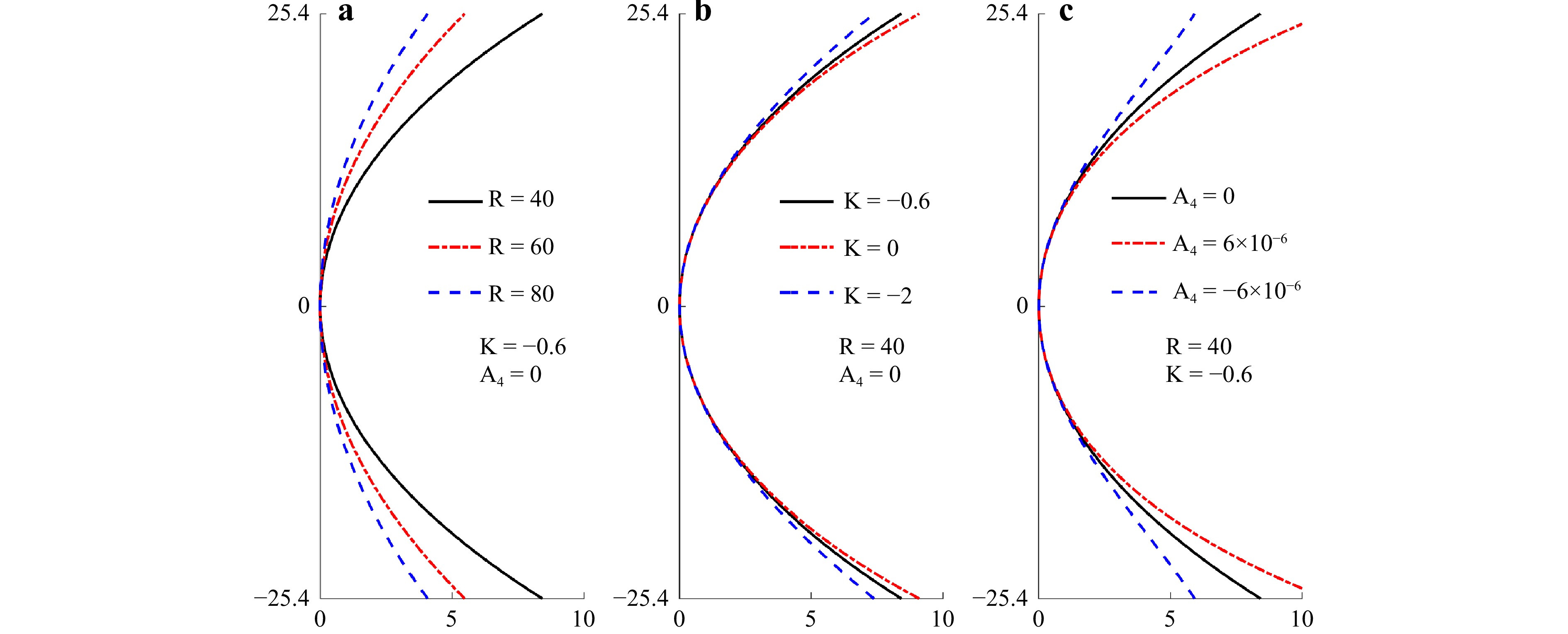
Fig. 1  Effects of ASPs on curvature: a vertex radius of curvature R, b conic constant K, and c high-order aspheric coefficients A_2i.

Surface form measurements are typically performed in the manufacturing of optical surfaces. Surface form measurement yields the deviation in the spatial domain between the surface under test and the design model, which can effectively guide processing in an optical shop. The peak-to-valley (PV) and root-mean-square (RMS) errors are generally adopted in surface form measurements to assess the quality of a single surface under test and can indicate the processing precision of the surface under test.

However, in an optical shop, assigning the exact final processing precision of each surface using only the PV and RMS errors of an aspherical optical system is challenging. Theoretically, an optical system can meet the requirements as long as the PV and RMS errors of each surface are sufficiently small. However, extremely small PV and RMS errors are rarely required for each surface because such an excessively high processing target will increase the cost significantly. Moreover, aspheric surfaces with excessive PV and RMS errors may form satisfactory systems in practice. The discussion above shows that the surface form measurement of each surface is insufficient for describing the performance of an optical system. Thus, assigning the exact final processing precision target to each surface using only PV and RMS errors is difficult. Hence, another measurement that can reflect the modulation of each light surface should be performed to evaluate the entire system.

In the context of optical system assessments, parameter measurement is an essential step in the manufacture of optical systems as it yields the light modulation deviation (e.g., the focal length change owing to curvature variations, as shown in Fig. 1) between the surface under test and the design model. This allows us to effectively assess whether the surface can function as expected in the optical system. For example, the measurement results of R can provide feedback to the model of an aspherical optical system in commercial optical design software to determine whether the focal length satisfies the requirements before the system is assembled. Moreover, the tolerance analysis of R can offer an exact processing target for aspheric surfaces prior to processing.

The parameter is a concrete form of the surface form in terms of the specific modulation of light. The surface form measurement yields the deviation in the spatial domain and can effectively guide the processing, whereas the parameter measurement can successfully assign the processing target of each surface by assessing the system performance degradation. A routine, cost-effective, and timely metrology solution for manufacturing aspheric surfaces is based on a reasonable combination of these approaches.

ASPs are highly demanded in modern advanced optical systems for ensuring good system performance. For example, the R of the primary mirror of the Giant Magellan Telescope is required to be R = 36,000.0 ± 1.0 mm³⁸, the R of the primary mirror of the James Webb Space Telescope is required to be R = 15,879.722 ± 1.0 mm, and the conic constant is required to be K = −0.9967 ± 0.0005 mm³⁹. Therefore, the measurement accuracy should be higher than the abovementioned fabrication accuracy. In this case, the measurement results of the ASPs can offer a vital reference for aspheric processing, thus providing guidance for the following processing steps as well as feedback on possible errors in the processing equipment.

Moreover, Eq. 1 is not the only expression used for the aspheric surfaces. The aspheric surface expressed in Eq. 1 is known as ‘even asphere’ in some commercial optical design software, such as Zemax. An extended version of Eq. 1 with a complete power series is known as ‘odd asphere’, which is expressed in Eq. 2.

The typically performed characterisation of rotationally symmetric aspheric surfaces adds a high-order power series to the conic surface. This representation is simple and provides substantial freedom in optical design. Theoretically, this representation can characterise any symmetric surface with arbitrary accuracy if i is sufficiently large⁴⁰. Nevertheless, this representation has been reported to be numerically deficient, and the non-orthogonality of the power series introduces considerable difficulty in the least-squares fitting of ASPs^40,41.

Forbes^40,42-44 proposed Q^con and Q^bfs polynomials based on Jacobi polynomials to address the challenges above. The Q^con polynomial was proposed for characterising a strong aspheric surface with large aspheric deviations and represents the aspheric deviations in the z-direction between the strong asphere and its conic base^45,46. The Q^con surface is generated by combining a conic base and the Q^con polynomial with an orthonormal amplitude. The expressions for a Q^con surface is shown in Eq. 3.

In Eq. 3, w is the normalised surface height and is defined as w = h/h₀, where h₀ represents the upper limit of h, B_i is a coefficient, and $ Q_i^{{\text{con}}} $ is a polynomial term³⁷.

The Q^bfs polynomial was proposed for characterising a mild aspheric surface with a constrained slope and represents the aspheric deviations in the normal direction of the best-fit sphere^45,46. The best-fit sphere matched the sag of the aspheric surface at the vertices and edges. The Q^bfs surface can enhance the manufacturability of an aspheric surface and is generated by combining a spherical base and the Q^bfs polynomial, which contains orthonormal derivatives. A Q^bfs surface is expressed as shown in Eq. 4.

In Eq. 4, C_i is a coefficient, and $ Q_i^{{\text{bfs}}} $ is a polynomial term³⁷. Moreover, the Q^bfs surface can be generated by combining a conic base and the Q^bfs polynomial as follows:

The aspheric surface types are listed in Table 2. An aspheric surface is typically generated using a quadratic surface, power series term, or Q-type polynomial. The ASPs include the vertex radius of curvature R, a conic constant K, and higher-order coefficients A_2i, A_i, B_i, and C_i. This review primarily focuses on even asphere because it is the most commonly used. In this case, ASPs include vertex radius of curvature R, conic constant K, and high-order coefficient A_2i.

Over the past few decades, methods for measuring ASPs have emerged to satisfy the increasing demand for various optical systems. However, the relevant reviews are currently unavailable. This paper reviews various techniques for measuring ASPs, which we hope will contribute to advancements in the fabrication and testing of aspheric optical elements and their practical applications in diverse fields.

The two core issues for a metrology solution are as follows: where data comes from and where data goes. The phrases ‘where data comes from’ and ‘where data goes’ refer to the measurement data source and the data processing approach, respectively. In many research areas, measurement techniques are typically classified based on the measurement data sources, which are directly related to the measuring instrument; therefore, the classification method is highly intuitive and informative. Meanwhile, unlike conventional physical quantities such as length and weight, ASPs cannot be directly quantified by measuring instruments. Therefore, research on ASP measurement is extremely diverse. Classifying ASP measurement methods using measurement data sources is difficult, and no clear classification exists currently.

Therefore, the ASP measurement methods presented herein are classified into two main categories based on the data-processing approach: general fitting and center-of-curvature-based methods. If the measured data are directly used to calculate the ASPs, then the method is classified as the general fitting method. If the measured data are used to position the corresponding centre of curvature, then the method is classified as the center-of-curvature-based method. In the center-of-curvature-based method, ASPs are typically calculated based on the distance between the local surface and the corresponding centre of curvature. Subcategories are then classified using a measurement data source.

This paper presents the basic principles, implementation schemes, and exemplary results of the different approaches. A summary and future outlook on techniques for measuring ASPs are provided at the end.

General fitting methods can be classified into the following three types based on the measurement data source: 1) the direct fitting method (surface form), 2) the interferometric method (wavefront aberration), and 3) the geometrical method (surface slope).

The direct fitting method is typically used to measure ASPs and is introduced in Section 2.1. It includes the following three important aspects: absolute surface form measurement, polynomial, and fitting algorithm. It is worth noting that though the surface form measurement is typically measured using an interferometer, the results obtained cannot be applied in the direct fitting method. This is because interferometry is a relative measurement method that can only yield the surface form deviation between the measured and reference surfaces, i.e., it cannot yield the absolute surface form. The technology for measuring the aspheric surface form is relatively mature. Related issues have been discussed by other scholars^2,47-52 and will not be discussed further herein. Section 2.1 introduces the polynomials and fitting algorithms for ASPs.

Accurate measurement of the aspheric surface form is expensive and inefficient. Therefore, other methods have been devised to measure the characteristics of light modulated by a surface instead of directly measuring the aspheric surface form. The phrase ‘characteristics of the light’ refers to a non-null system wavefront, longitudinal aberration, spot deviation, or other measurable quantity. Complex formula derivations and optical path parameter measurements are typically required prior to ASP fitting. These methods are introduced in Sections 2.2 and 2.3 based on the type of measured characteristics.

In the direct fitting method, a coordinate measuring machine^53,54, a swing arm profilometer^55-57, a Hartmann sensor^58,59, a scanning white light interferometer⁶⁰, or other instruments^61-72 are used to measure the aspheric surface form. Subsequently, the measured data are mathematically fitted to obtain the ASPs. A typically used mathematical fitting process is described as follows^73,74:

Determining the best fit for a model function F to a set of measured data F_n with N data points typically requires a minimisation process. A model function F can generally be expanded by a polynomial P of degree I as follows:

This process can be described as obtaining coefficients A_i to minimise the merit function M, which is expressed as

In Eq. 7, M is a quadratic function of coefficient A_i. According to the extreme value theorem, if M is a differentiable function, then the minimum is obtained when the partial derivatives of the function for each coefficient are zero.

This implies that for Eq. 7,

for all i =0,1, 2, …, I, and J = I. Resolving this equation yields

Thus, the following can be obtained at each minimum:

Subsequently, the variables below are introduced:

Hence, Eq. 11 becomes

and can be expanded as

Eqs. 13, 14 are the normal equations of the least-squares data fitting problem: If the determinant of G does not vanish, then a unique set of solutions A₁, A₂, …, A_i exists. This equation can be easily obtained using the classical least-squares matrix inversion method⁷⁵.

Eq. 6 can be represented in matrix form as

Subsequently, the following can be obtained using the least-squares matrix inversion method:

a. Challenges in conventional least-square direct fitting method

As shown in Eq. 16, the least-squares matrix inversion method inverts the Gram matrix G = P^TP, which results in numerical instability in the high-order power series fitting process⁷⁶.

Forsythe⁷³ used regression theory to show that the aforementioned least-squares matrix inversion method is computationally intensive and utilised a typical numerical model to illustrate the strict tolerance of the method under high-order conditions. When N is large and P (x_n, y_n) is distributed approximately uniformly on (0, 1), one may expect

In this case, matrix G is N times the matrix [[(i + j + 1) ⁻¹] (i, j = 0, 1, …, k), which is the well-known principal minor of order k + 1 of the infinite Hilbert matrix.

Solving linear equations involving the minor components of H is difficult. For example, for k = 9, the order of the principal minor H₁₀ is 10 and the inverse H₁₀⁻¹ contains elements of magnitude 3 × 10¹². In this case, a slight error of 10⁻¹⁰ in c_i results in an error of approximately 300 in A_i, indicating that the solution to Eq. 16 is highly sensitive to errors in F_n ⁷³. The simplistic fitting process fails when the terms are in excess, owing to the strict tolerance. However, if I is specified within a certain range, the number of terms will be reduced, resulting in the inability of the expression to adequately describe the aspheric surface.

The discussion above indicates that the performance stability of the least-squares matrix inversion method depends significantly on the Gram matrix G, which is determined by the polynomial set P. The spectral condition number κ can determine the condition of G.

where σ(G) denotes the set of all eigenvalues of G. Condition values of approximately 1 indicate that G is well-conditioned, whereas high values indicate that G is ill-conditioned⁷⁴.

In the fitting process using the least-squares matrix inversion method and the power series in Table 1, massive coefficients can be obtained when the peak polynomial coefficient increases with the polynomial order. These coefficients are typically several orders of magnitude higher than the sagittal height. This condition may result in a remarkably small number from the subtraction of two large numbers during the sagittal height calculation. Thus, the effective numbers during the calculation decrease because of the limited accuracy of numerical storage in computers. The loss of effective numbers induces numerical instability in the optimisation algorithm used in the calculation. This problem of fitting ASPs can be solved using polynomials and fitting algorithms.

b. Polynomials

An orthogonal polynomial can sufficiently eliminate the numerical instability of the fitting algorithm during the calculation. Forsythe remarked that setting G_ih (i ≠ h) to be substantially smaller than the diagonal elements of G_hh will significantly simplify the solution to Eq. 14 for large values of polynomial degree I⁷³. A typical practice is to select polynomials that are orthogonal to the dataset as follows: x₁, x₂, …, x_N. Owing to the discrete orthogonality condition, if the polynomial set P_i is orthogonal, then

and the simple form of Eq. 14 can be obtained as follows:

Thus, the coefficients for the best fit can be easily calculated as follows:

Instead of a simple additional power series, Forbes^40,42-44 used a nonstandard orthonormal basis in the aspheric expression formula to avoid an ill-conditioned Gram matrix and proposed three types of function polynomials: Q^con, Q^bfs, and Q^bfs extended. The Q^con and Q^bfs polynomials are typically used to characterise symmetrical surfaces, as listed in Table 1. Q^bfs extended polynomials are used to define complex surface shapes with local protrusions or depressions and can be extended to characterise freeform surfaces. However, Q-type polynomial is defined as orthogonal over continuous data and may not be orthogonal for discrete data. Meanwhile, data obtained from actual tests are typically discrete. Hilbig et al.⁷⁴ proposed the Gram-Schmidt orthonormalization of these polynomials over a discrete dataset to solve this problem. Wang et al.⁷⁷ expanded the quadratic portion of an aspheric surface into a series of even-order terms using binomial expansion to generate discrete orthogonal polynomials. The definition of the fitting error is directly related to the inner products; therefore, Cheng et al.⁴¹ projected polynomials to the vector space based on their relationship with the inner products. Polynomials were analysed using vector analysis methods, where polynomial problems were transformed into vector problems. This method can achieve high accuracy and effectively solve numerical ill-conditioning problems.

c. Fitting algorithms

The fitting algorithm determines the performance and efficiency of the direct fitting method. Herein, the main list of fitting algorithms applied to ASP fitting is presented. Zhang⁷⁸ (1997) derived aspheric parameter fitting comprehensively and compared various algorithms. The parameter estimation problem was regarded as an optimisation process. A comprehensive discussion of the minimisation criteria and the robustness of the different algorithms was provided. The importance of selecting an appropriate criterion was highlighted as it can affect the accuracy of the estimated parameters, the computation efficiency, and the robustness to predictable or unpredictable errors⁷⁸. Gugsa⁶⁰ (2005) used the least-squares method to determine the best-fit conic of aspheric microlenses based on white-light interferometry, where the Monte Carlo process was used to estimate the measurement uncertainty of the test results. Sun⁷⁹ (2009) utilised the Gaussian–Newton algorithm to fit aspherical curves and surfaces by minimising the vertical distances. This fitting process converged rapidly in the simulated ideal data and data containing random irregularities. In the same year, Chen et al.⁸⁰ discussed the form-fitting of rotationally symmetric aspheric surfaces using the least-squares method and the Levenberg–Marquardt algorithm, which resulted in rapid convergence. El-Hayek⁸¹ (2014) evaluated the following three algorithms based on their performances on simulated datasets: the limited memory Broyden–Fletcher–Goldfarb–Shannon (L-BFGS) algorithm, the Levenberg–Marquardt algorithm, and one variant of the iterative closest point algorithm. The L-BFGS algorithm showed linear time complexity with respect to the number of data points, executed faster than the Levenberg–Marquardt algorithm, and was significantly faster than the iterative closest point algorithm.

In general, the direct-fitting method exhibited good versatility. However, the direct use of a non-orthogonal power series for fitting high-order aspheric surfaces causes numerical instability in the calculation. Robustness and efficiency are prioritised in fitting algorithms. A fitting algorithm is susceptible to non-convergence when the number of fitting points is small. The efficiency of fitting algorithms for addressing large-volume datasets garnered considerable attention. Therefore, researchers have focused on different orthogonal polynomials as well as rapid and accurate fitting algorithms.

Interferometry is an efficient optical method that is widely used to test optical aspheric surfaces^{10, 47, 82-88}. This method requires a compensator to reduce the maximum slope of the residual wavefront of the interferometry system; thus, the density of the interference fringes satisfies the Nyquist theorem. The compensator converts the aspheric wavefront into a spherical or plane wavefront, the latter of which interferes with the reference wavefront. Interferograms are analysed to obtain the target information of the aspheric surface under testing (ASUT). Interferometric measurement methods involving a compensator can be classified into null and non-null interferometry based on the compensator type^49,89-98.

Null interferometry adopts a null compensator or computer-generated hologram (CGH), which generates a wavefront consistent with the ASUT to compensate for the normal aberration of the aspheric surface, thus allowing a null interferogram to be obtained^82,83. This method can achieve high accuracy; however, a null compensator or CGH can only measure a specific aspheric surface, thus significantly increasing the manufacturing costs. The null interferometric measurement system requires the precise positioning of the ASUT at the confocal position of the measurement system, thereby increasing its complexity. In addition, the manufacturing and testing of the null compensator or null CGH is complex, which limits the wide application of null interferometry for ASPs.

Non-null interferometry is widely used to measure ASPs. As shown in Fig. 2, the typical non-null interferometry uses a partial compensator (PC) to construct a partial compensation interference system^49,92,99. A PC can be used to test a series of aspheric surfaces, thereby reducing the measurement costs and improving the versatility. Unlike null interferometry, non-null interferometry features a large residual normal aberration in the system wavefront, which is known as the residual wavefront, thus resulting in a retrace error that must be corrected. The residual wavefront is related to the compensation distance, which is defined as the distance between the final surface of the PC and the vertex of the ASUT¹⁰⁰. The compensation distance is important and was adopted widely in previous studies.

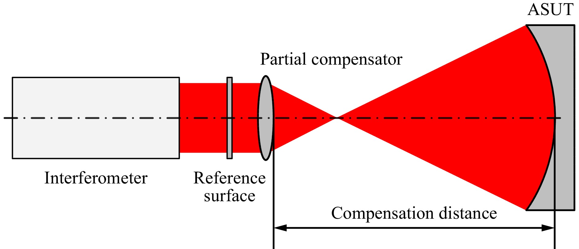
Fig. 2  Definition of compensation distance

Yang et al.¹⁰¹ proposed a measurement method for R of an aspheric surface using a non-null interferometry system. As shown in Fig. 3, this method uses the multi-configuration of a non-null interferometer for optimisation and can simultaneously yield the R and surface form of the ASUT. An aspheric shift with precisely determined axial displacements was conducted to realise multiple measurements, and a multi-configuration model was established accordingly. The R and aspheric surface error were entered into the multi-configuration model as variables, whereas the experimentally tested residual wavefronts were regarded as optimisation objectives. Subsequently, the actual R was retrieved via a simultaneous optimisation process. Theoretically, the accuracy of the results can be improved by increasing the number of measurements. Nevertheless, such improvements typically require additional complex operations and present cumulative errors. The computational efficiency of this method relies on the estimation of the initial value of R and the initial position of the measured aspheric surface. The relative measurement accuracy of this method can exceed 0.025% when measuring a paraboloid mirror with a nominal R of 819.52 mm.

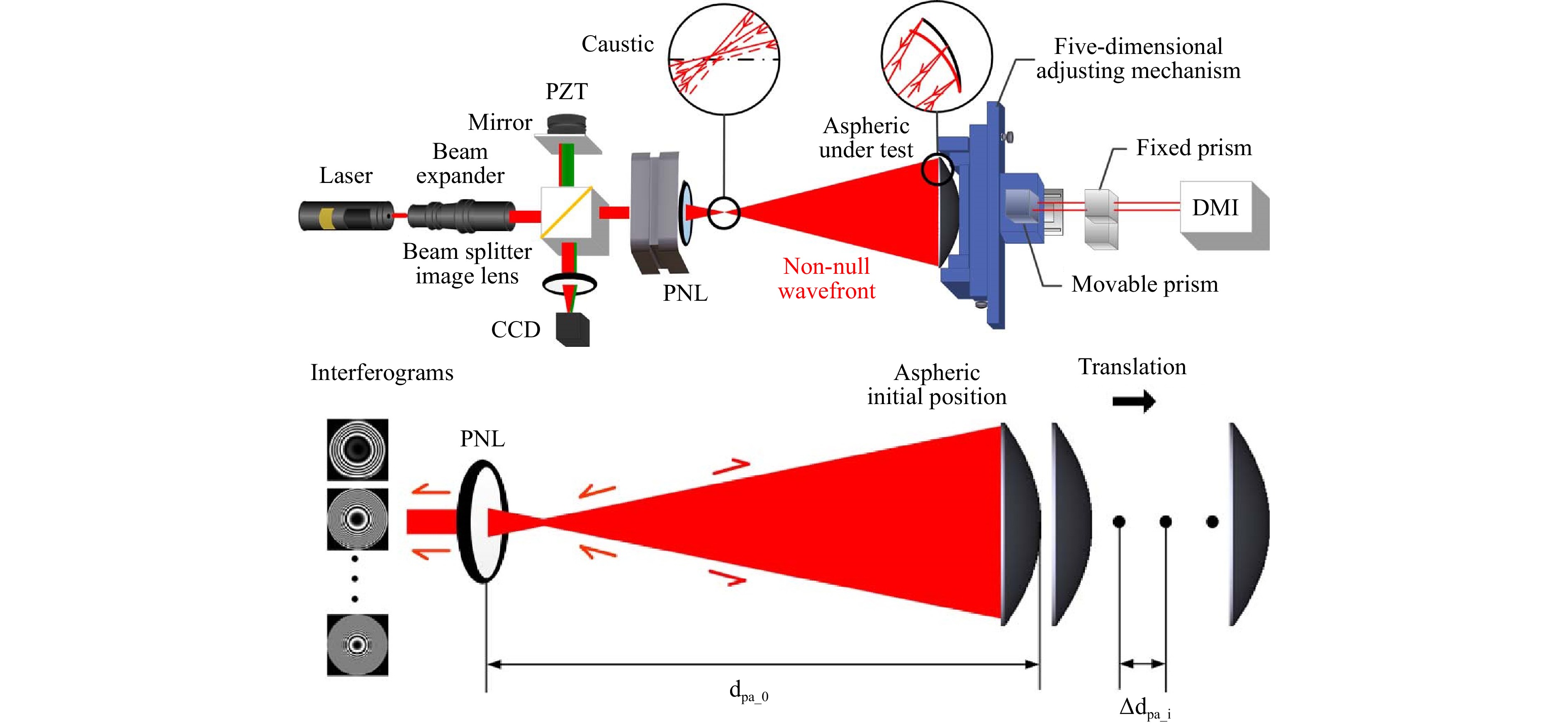
Fig. 3  Schematic illustration of aspheric non-null interferometry for different axial positions (Reprinted with permission from Ref. 101 Ⓒ Optica Publishing Group)

The measurement of R using the introduced method does not rely on the absolute positioning of the confocal position or the absolute value of the compensation distance, thereby reducing the adjustment difficulty. In fact, this method is applicable to the measurement of R for annular aspheric surfaces. However, its requirements for accurate axial displacement measurements and for fitting rotationally symmetric aberrations in the measured wavefront are high, and neither K nor A_2i is measured.

Hao and Hu et al.^{91, 92, 99, 100, 102-104} comprehensively developed non-null interferometry to measure ASPs both theoretically and experimentally.

First, a new concept known as the best compensation distance was defined to assist the measurement^100,102. In a non-null measurement system, the maximum slope of the residual wavefront changes as the aspheric surface propagates along the optical axis. When the maximum slope and density of the interference fringes reaches the minimum value, the compensation distance is defined as the best compensation distance. This position can be identified by observing the density of the interference fringes. The system wavefront obtained at the best compensation distance is the best compensation wavefront.

Subsequently, a mathematical model is established to define the relationship among the ASPs, system wavefront, and best compensation distance. By considering the McLaurin series expansion of Eq. 1, z can be expressed as shown in Eq. 23.

The relationships between the ASPs and system wavefront are as follows¹⁰³:

Eq. 24 establishes the relationship between the best compensation wavefront deviation and errors in the ASPs. In this equation set, ΔD_2i is the difference between the coefficients D′ and D of the actual and theoretical aspheric surfaces; ΔR, ΔK, and ΔA_2n are the errors in ASPs; and Δφ is the deviation between the actual best compensation wavefront φ′ measured in the actual non-null interferometer and the ideal best compensation wavefront φ. Nevertheless, in this equation set, ΔD_2i can be calculated from the last equation while ΔR, ΔK, and ΔA_2i (i = 2, 3, and 4) are unknown. A total of i equations and i + 1 unknown quantities are involved. Therefore, the equations are undetermined and have infinite solutions. Similar to the best compensation wavefront, the best compensation distance changes when an error is observed in the ASPs. Another equation can be established by describing the relationship between the deviation of the best compensation distance and the error in the ASPs¹⁰³. The detailed equation is complex and is omitted herein.

Finally, measurement methods for the best compensation distance remain unknown. Unlike a spherical interferometry system, a non-null system does not have a cat’s eye or confocal position. Therefore, measuring the best compensation distance, which is key to the entire system, is difficult.

This issue can be mitigated by adding a removable combined aplanat to the PC, as shown in Fig. 4, to locate the cat’s eye position^100,105. The layout of this approach is illustrated in Fig. 5. The distance between the PC and the cat’s eye position can be obtained easily based on the aplanat design. After locating the cat’s eye position, the combined aplanat is removed and the aspheric surface propagates along the optical axis on a precision linearity rail to the position where the density of the interference fringes reaches the minimum to calculate the best compensation distance. However, determining the precise location of this position is difficult because the interferogram fringes are similar near the target position. Thus, an iterative optimisation algorithm is utilised to calculate the real best compensation distance and ASPs. The relative measurement accuracies of R and K yielded by this method exceed 0.02% and 2%, respectively, for a conic surface¹⁰⁴.

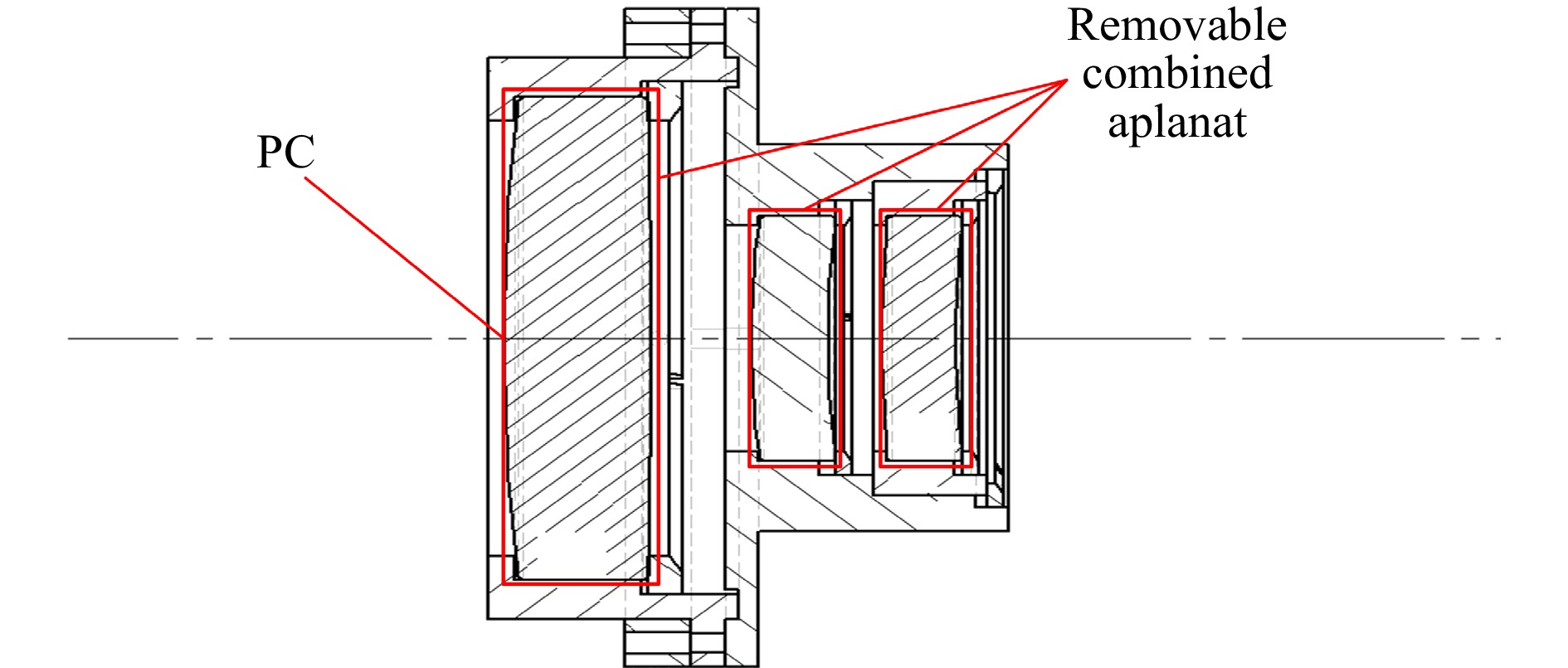
Fig. 4  Layout of removable combined aplanat (Reprinted with permission from Ref. 100 ⓒ Optica Publishing Group)

Fig. 5  Layout of non-null interferometry with removable combined aplanat (Reprinted from Ref. 104, with the permission of AIP publishing)

However, the versatility of this approach is insufficient. Different aplanats must be designed for various PCs to eliminate spherical aberrations, thus increasing the test cost. The ASUT must traverse a long distance of approximately the R of the ASUT, which is time-consuming and risky when measuring a large optical element. The accuracy of the guide rail limits the precision of the compensation distance measurement. Theoretically, this approach can be extended to measure A_2i; however, further study is required for confirmation.

The laser differential confocal technique was used in another study to measure the best compensation distance¹⁰³. A schematic illustration of this approach is shown in Fig. 6. The system can be classified into two subsystems: the partial-compensation interferometer system (which is enclosed by the solid line) and the laser differential confocal system (which is enclosed by the dashed line). The real partial compensation interferometer system measures the system wavefront, whereas the laser differential confocal system measures the best compensation distance. The compensation distance is adjusted until the PV value of the residual wavefront reaches the minimum. The wavefront of the system is obtained using a Fizeau interferometer. The PC and ASUT are mounted together to fix the compensation distance. Subsequently, the best compensation distance can be measured after moving the compensator and ASUT to the laser differential confocal system integrally. This approach increases the measurement accuracy of the compensation distance and the versatility of non-null interferometry, thus allowing high-order aspheric surfaces to be measured, and is suitable for measuring concave and convex aspheric surfaces. The relative accuracies of R, K and A_2i can reach 0.025%, 0.095%, and 3.02%, respectively.

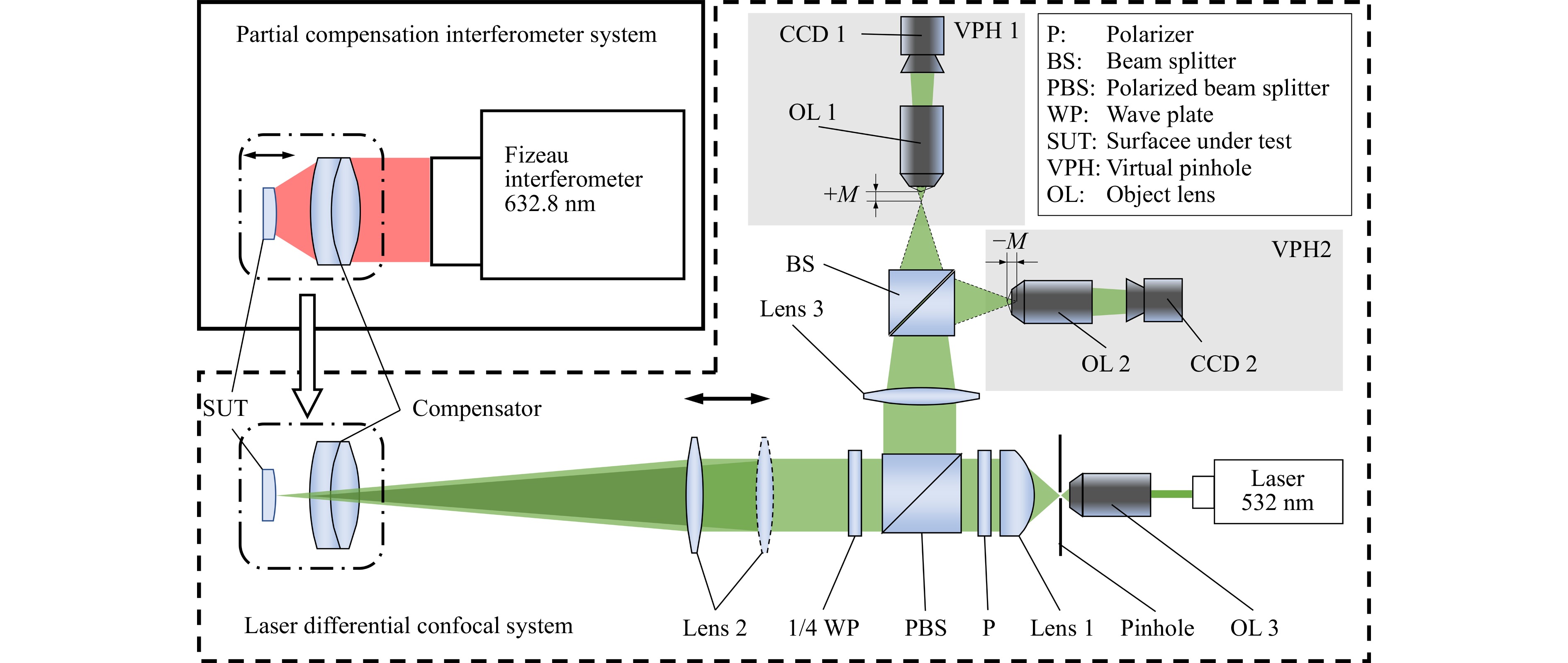
Fig. 6  Schematic illustration of non-null interferometry based on laser differential confocal technique (Reprinted with permission from Ref. 103 ⓒ Optica Publishing Group)

In this method, the PC and ASUT should be fixed and propagated between the interferometer and laser differential confocal system, which is not feasible when testing large optical elements.

In general, the interferometric method can achieve high accuracy in surface form measurements. The information retrieval of this method is based on light wavelength, thus providing superior traceability to the test results. This method requires a compensator to convert the reference wavefront into an aspheric wavefront, and using multiple compensators enable the comprehensive measurement of various convex or concave aspheric surfaces.

The ASPs were calculated by establishing relationships among the ASPs, system wavefront, and compensation distance. Nevertheless, the measurement of the compensation distance does not satisfy the test requirements in various test scenarios. The aplanat approach requires the propagation of the ASUT over long distances. The laser differential confocal technology system is complex, where the ASUT and PC must be fixed and propagated. Implementing these conditions in tests for optical elements with a long R or large diameter is typically difficult. Therefore, a compensation distance measurement method that can satisfy different application scenarios is urgently required.

For interferometry systems, the setup is complicated and the measurement range is relatively small. Furthermore, interferometry cannot correctly retrieve the wavefront when the ASUT presents a height discontinuity greater than one-quarter of the light wavelength between two adjacent pixels. Additionally, the 2π phase ambiguity appears in an unwrapped operation¹⁰⁶. These conditions limit the applicability of interferometric methods.

Geometrical methods are cost effective and have been widely used to test the surface form of optical elements^{58, 59}, such as via the Hartmann test. Unlike interferometric methods, a geometric optics approach measures the slope from transverse aberrations at some observation planes near the focal plane instead of the optical path difference¹⁰, thus avoiding the 2π phase ambiguity problem. Thus, this method has a wide measurement range.

Diaz-Uribe et al. (2000)⁶² proposed a null-screen method for testing fast-aspheric convex surfaces. Fig. 7 shows the mechanism of this method, which uses a cylindrical screen with a set of stripes, dots, drops, or grids. An image is reflected by a perfect surface and a perfect image is created when the drop-null screen is adopted, as shown in Fig. 8a. Each screen is specifically designed to accommodate the ASUT. If the ideal form of the surface to be evaluated is known, then the observed image shown in Fig. 8b indicates the departure from a perfect array if the surface is not ideal. As shown in Fig. 8c, the differences between the theoretical and experimental arrays can be attributed to surface imperfections and can provide relevant information regarding the form of the surface to be analyzed⁷¹. As shown in Fig. 9, this method is simpler than other null-test methods in terms of structure because it does not require any additional optical elements with a specific design to correct the aberrations of the system under test. Slight deviations can be quantified in an image of the grid by measuring the x- and y-coordinates at each crossing point. Additionally, alignment can be performed easily because the setup is entirely along the local axes of each segment and the grid or other designed patterns allow the screen to be positioned easily.

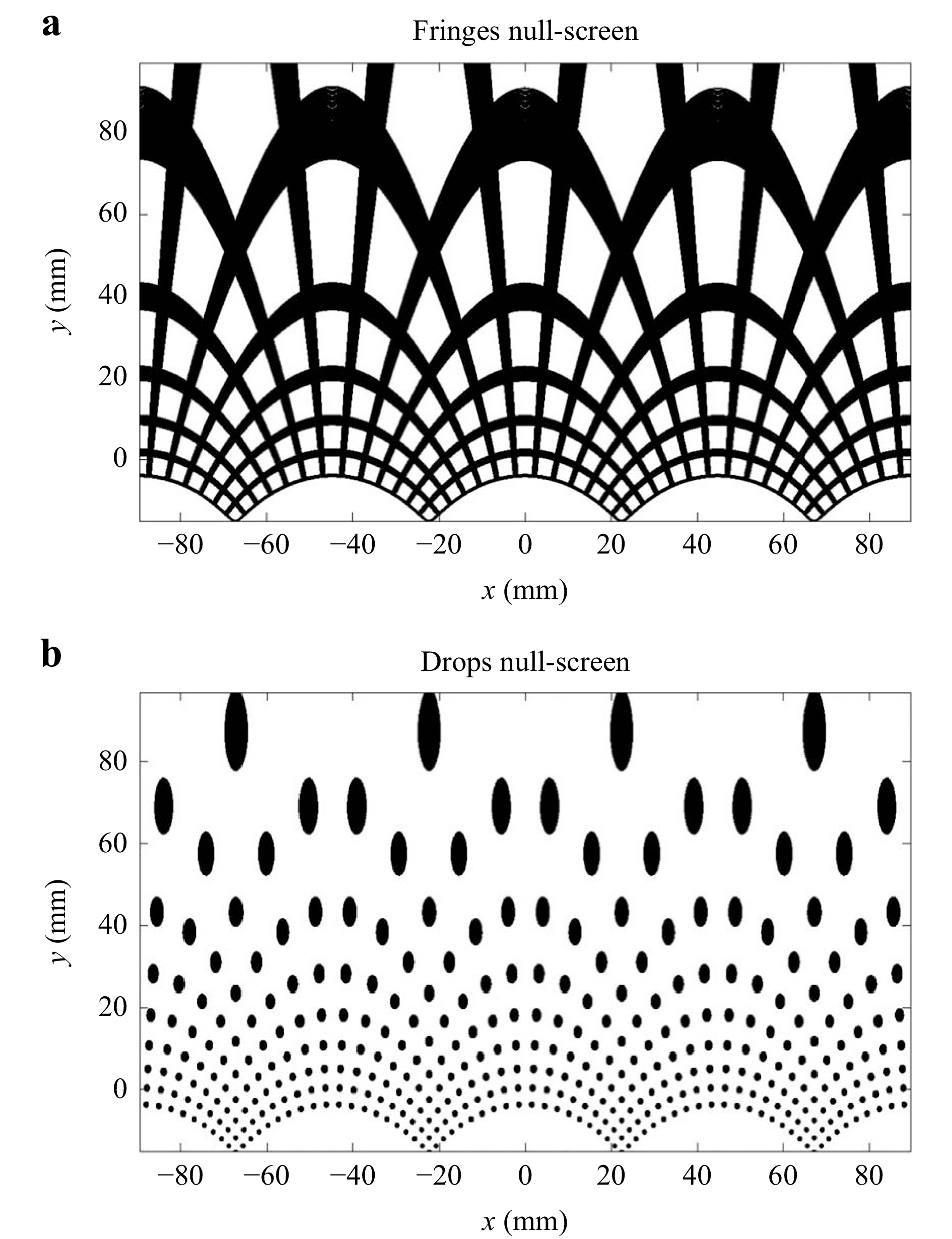
Fig. 7  Flat-printed null screen: a fringes and b drops. (Reprinted with permission from Ref. 71 ⓒ Optica Publishing Group)

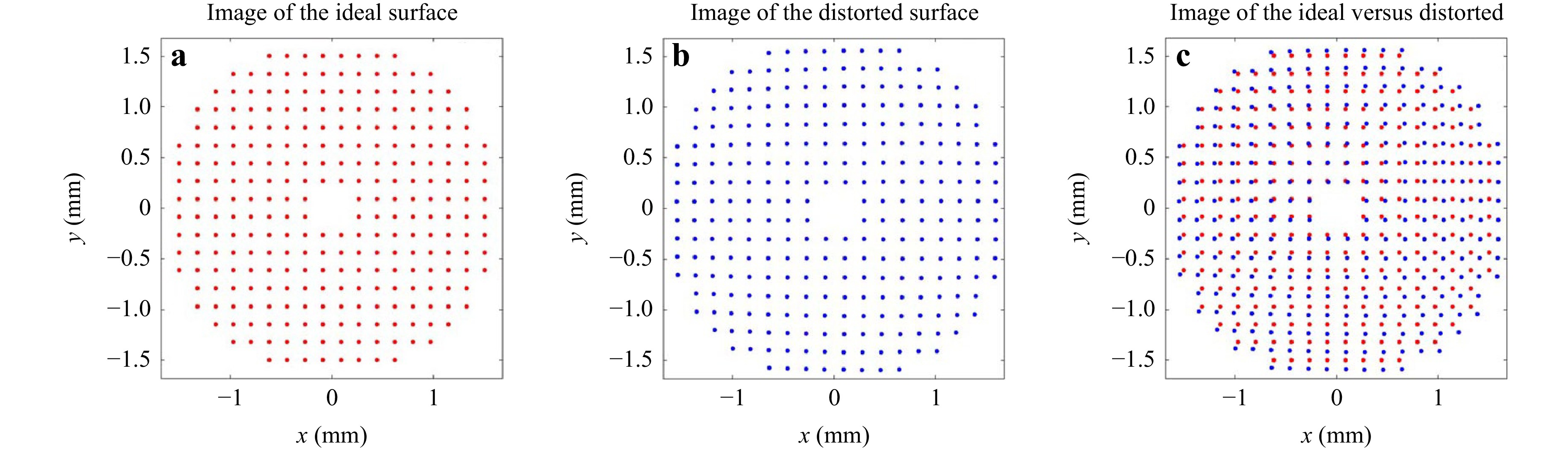
Fig. 8  Centroids on CCD: a theoretical, b distorted, and c comparison of a and b. (Reprinted with permission from Ref. 71 ⓒ Optica Publishing Group)

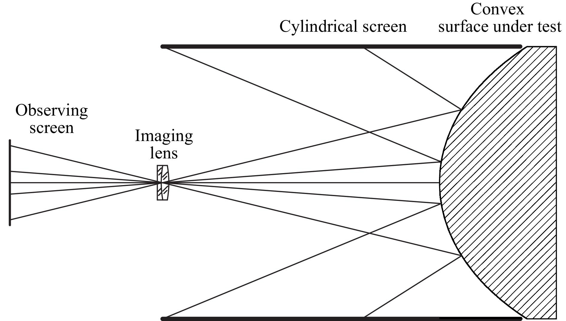
Fig. 9  Layout of null screen method (Reprinted from Ref. 10, Copyright ⓒ 2007 by John Wiley & Sons, Inc. All rights reserved)

This method was further developed and can be applied quantitatively to test convex and concave aspheric surface forms^64-72. Similar to the Hartmann test, this method involves a quantitative evaluation of the null-screen method via a numerical integration process, such as trapezoidal integration¹⁰, and accumulates errors along the integration path. Furthermore, it can be used to qualitatively test large surface departures by visually examining the grid image at the CCD, which is practical during the preliminary manufacturing step. Hence, the ASPs can be fitted when the surface form has been measured.

In addition to the direct fitting approach, the null screen method allows ASPs to be measured directly using novel algorithms. Aguirre-Aguirre et al.(2017)⁷¹ proposed a randomised algorithm to recover the R, K, and surface forms of their ASUT. In this approach, instead of performing integration and polynomial fitting, a direct and random process was used to determine the surface form. The process involved proposing a new test surface, where the R and K values of the surface are selected randomly, and the null screen was compared with the initially designed one. For the ASUT, R and K, which yielded a null screen that was the most similar to the reference null screen, were specified with the final values. Integration errors were avoided and thus the total error was reduced significantly. The relative accuracies of R and K were 0.4% and 0.5%, respectively.

Aguirre-Aguirre et al. (2018)¹⁰⁷ extended the method above to calculate a null screen to test fast convex/concave odd aspheric surfaces with high-order coefficients. This approach can extract the target parameters via a simple procedure; hence, a null-screen test can be conducted without unmounting the optical system from the polishing machine to test the form of the surfaces in the early stages of polishing, which demonstrates the efficiency of this method. The percentage error of this method was shown to be less than 1.3% for the recovery of high-order coefficients A_i.

Diaz-Uribe and Cornejo-Rodriguez^108,109 proposed the geometric method in the 1980s to measure the R and K of quadratic aspheric surfaces. The setup of this method, which comprises a goniometric table and a lens holder with a micrometric screw, is shown in Fig. 10. In this method, the longitudinal aberrations of the normals to the surface and their corresponding angles are obtained on the nodal bench to calculate R and K. The measurement principle is simple and easy to implement. This method is applicable even when the centre of the surface cannot be used but fails when the surface is extremely close to a spherical surface. The accuracy of this method barely satisfies the current test requirements but can be improved using precise auxiliary instruments.

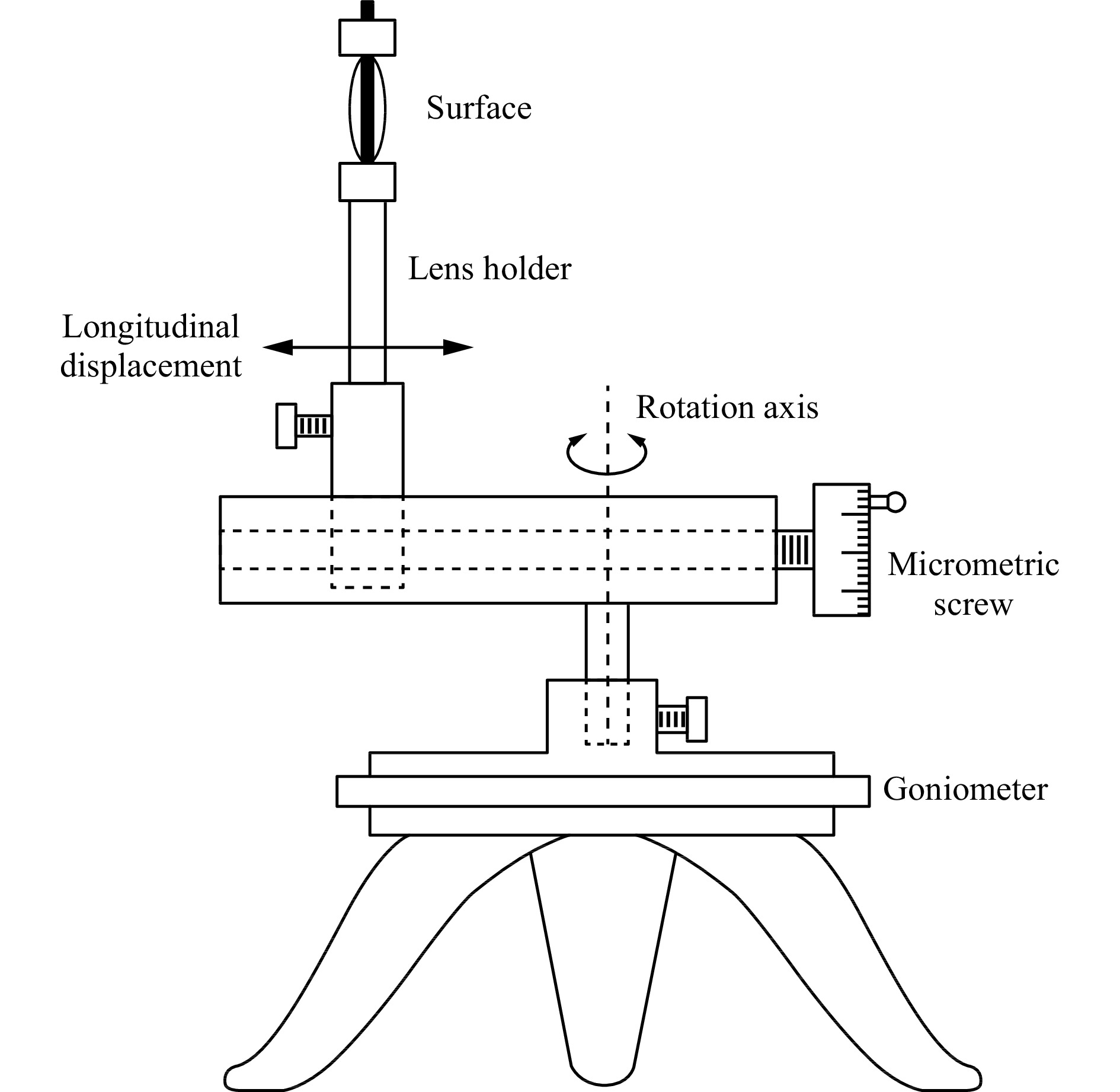
Fig. 10  Layout of nodal bench (Reprinted with permission from Ref. 108 ⓒ Optica Publishing Group)

Wang¹¹⁰ proposed a ray-tracing method to measure the R of aspheric surfaces. The principle of this method is illustrated in Fig. 11. In this method, spot-array rays generated by a laser and grating are projected onto the ASUT, and the positions and directions of the incident and reflected rays are recorded using two shifting receiving planes. A ray tracing method provides the equations for each ray and the coordinates of its intersection point with the surface under testing. Subsequently, measurements can be performed by applying a surface-fitting algorithm to determine the aspheric vertex locations and an optimisation algorithm to calculate the symmetry axis and curvature centre. This method involves a simple structure and can be used to test the R values of most aspheric surfaces. The relative measurement accuracy R exceeds 0.5%.

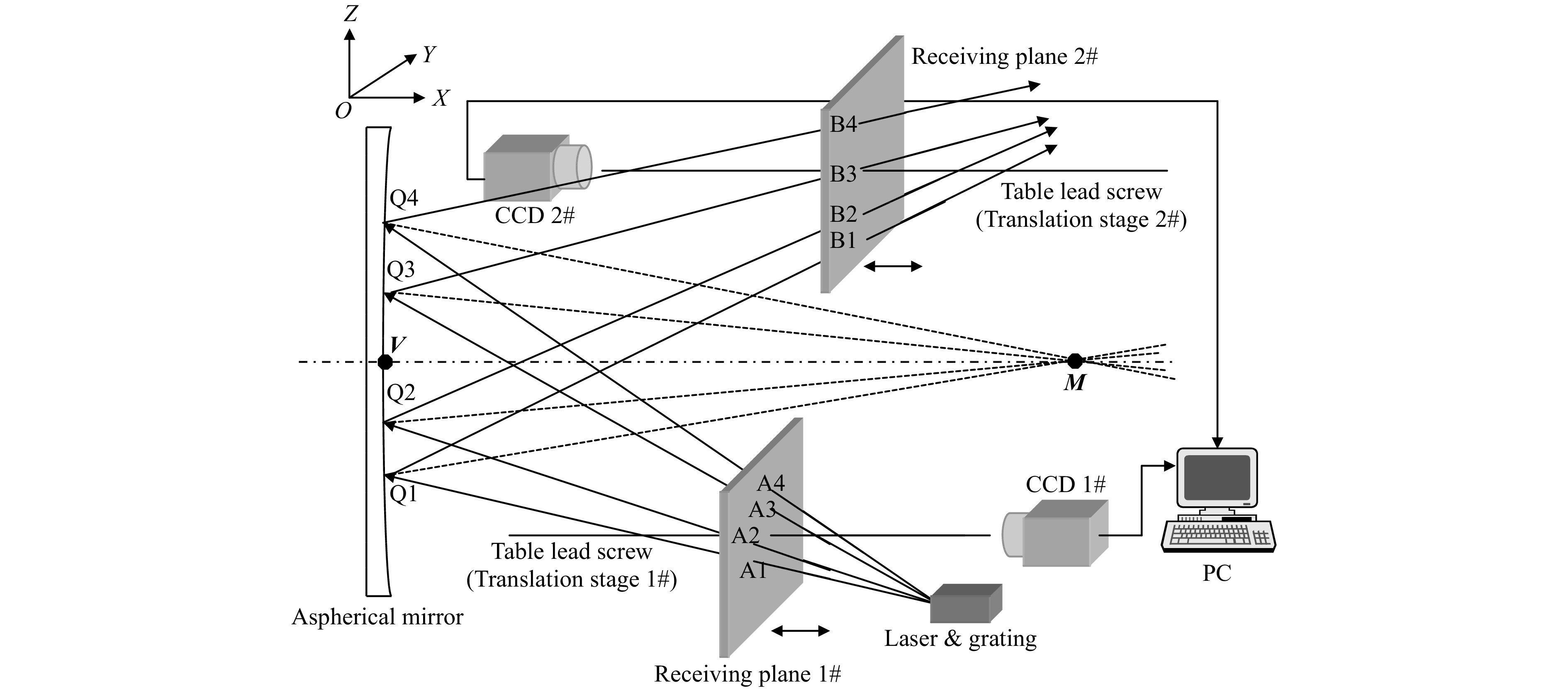
Fig. 11  Optical system of experimental ray-tracing method (Reprinted from Ref. 110, Copyright 2004, with permission from Elsevier)

In general, the geometrical method is simple in terms of structure and has a large measurement range. A numerical integration process can be applied to this method to obtain the surface form, and then the ASPs can be fitted. In addition to direct fitting, various algorithms and devices have been proposed to obtain the ASPs directly. A modified method based on a randomised algorithm that avoids integration errors and low spatial resolution problems can yield high performance. The highest relative accuracies of R, K, and A_i reached 0.4%, 0.5%, and 1.3%, respectively, when an odd aspheric surface was used as the ASUT.

A widely used radius measurement method for spherical optical elements is based on the centre of curvature of a spherical surface. This method identifies two null interferograms at two positions: the cat’s eye and confocal positions^111-113. The distance between the two positions is R. It is considered one of the most accurate methods for measuring R. In fact, this method can be extended to the measurement of ASPs by determining the centre of curvature or the focal point of the aspheric surface. An aspheric surface has features that are similar to those of a spherical surface. For example, the paraboloid can focus parallel light on its focal point without aberration; the hyperboloid comprises a pair of conjugate focal points, where the spherical wave emitted from one focal point converges to the other, and the compensator or CGH can yield the confocal position in the measurement of high-order aspheric surfaces. The positioning approaches used in this method are based on two physical principles: interferometry and laser differential confocal techniques. In particular, the ASPs are derived from the system wavefront obtained using the interferometer described in the previous section, whereas an interferometer is utilised to determine the position of the centre of curvature or the focal point.

Pi¹¹⁴ proposed a method for measuring R and K based on the wavefront aberration characteristics of an ASUT. The test setup is shown in Fig. 12. A convergent beam emitted by the transmission sphere of the interferometer yields a focus point at the cat’s eye position. An arbitrary region of a conic surface is aligned to the interferometer with the surface normal to the centre of the beam, coinciding with the interferometer optical axis. Fig. 12 shows that the three confocal positions can be identified using the corresponding characteristic interferograms, where the focus corresponds to the centre of the sagittal, medial, and tangential radii of curvature (R_T, R_M, and R_S, respectively) of the test region. The interferometer measures the optical path difference W between the test region on the surface and a spherical reference wavefront whose radius of curvature is equal to R_T, R_M, or R_S. The Seidel aberration coefficient is fitted from W and combined with the distance between the three specific positions and the cat’s eye position to calculate R and K. This method does not require knowledge regarding the position of the test region and can therefore be used on mirrors without fiducial markings, including those that are already mounted on a telescope.

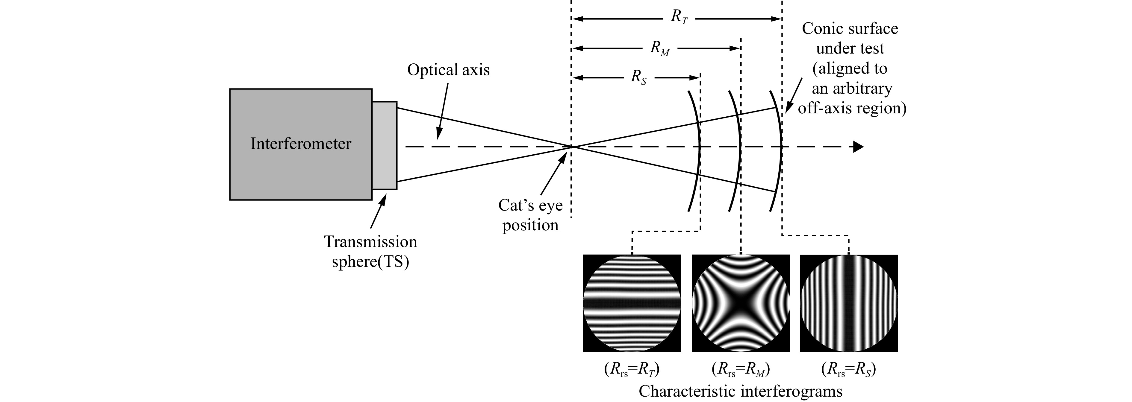
Fig. 12  Layout of off-axis segment method (Reprinted with permission from Ref. 114 ⓒ Optica Publishing Group)

Li and Chen et al. (2015)^115,116 used a null interferometry system to measure the R and K values of aspheric surfaces. As shown in Fig. 13, this method uses a portable laser tracker to measure the compensation distance and then determines R via ray tracing. K is calculated via a linear approximation between R and K when the axial deviation of the aspheric surface from the confocal position is slight. Experimental results of an asphere with R ~2 m show that the repeatability of R and K were ±0.039 mm and ±2.05 × 10⁻⁵, respectively.

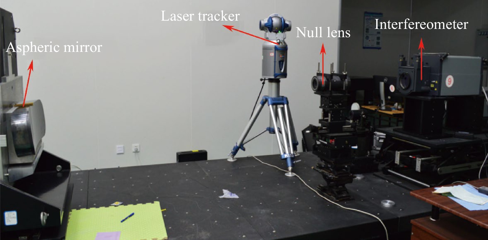
Fig. 13  Experimental setup for null interferometry using a laser tracker (Reprinted from Ref. 116, with permission from Chinese Laser Press)

In the aforementioned interferometric methods, ASPs are fitted using the system wavefront obtained from the interferometer. The interferometer used in this method provides only the criterion for confocal positioning. This method is similar to the conventional interferometry for measuring the radius of a spherical mirror. The mechanical exterior cylindrical surface and backplane of the compensator are set as the reference surfaces and processed with high precision when the laser tracker is used to measure the compensation distance. In addition, a centration test device is required to align the compensator to ensure correspondence between the reference surface and main optical axis.

Yang (2014)¹¹⁷ proposed a laser differential confocal measurement method for measuring the R value of a paraboloid. The test setup is illustrated in Fig. 14. In this method, an autocollimation R measurement light path is constructed by placing a flat mirror as a reflector on the incident light path. Positions A and B with axial coordinates z_A and z_B correspond to the test paraboloidal focus and vertex, respectively. The distance between positions A and B determines R = 2(z_A − z_B). This method can precisely determine positions A and B using null points Q_A and Q_B derived from the corresponding differential confocal response curves I_A and I_B, respectively. Its uncertainty in measuring R is less than 0.001%.

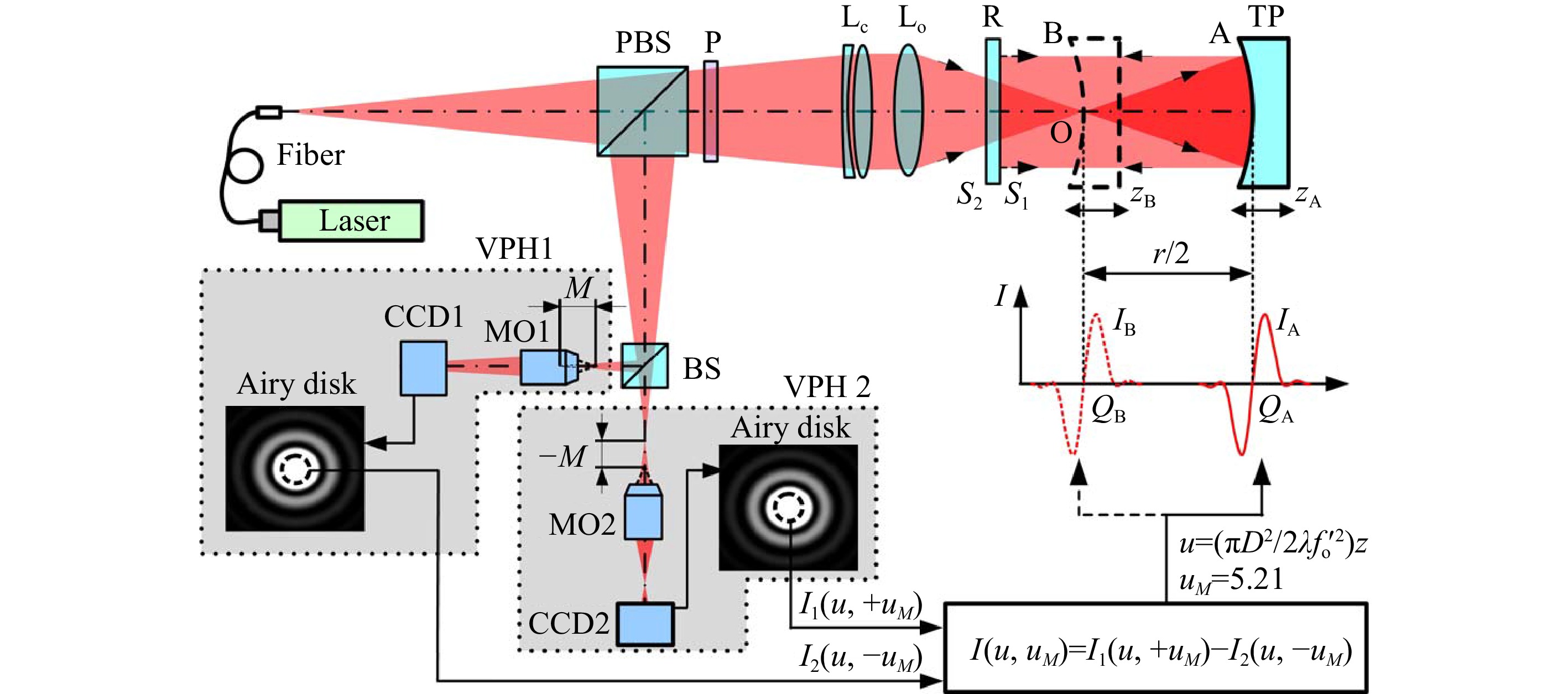
Fig. 14  Principle of laser differential confocal technique (Reprinted with permission from Ref. 117 ⓒ Optica Publishing Group)

This method is highly accurate, efficient, and insensitive to environmental disturbance^118,119. Furthermore, it can be applied to measure the R of other aspheric surfaces via an appropriate compensation technology. However, this method cannot measure the K and A_2i values of aspheric surfaces. By default, the ASUT presents an error in only R, not in K. The errors in K affect the measurement accuracy of R.

In general, the center-of-curvature-based method has a significant advantage in measuring R but can only be applied in the test of conic surfaces. R can be measured accurately by identifying specific axial positions using interferometry or laser confocal differential techniques. The achievable maximum relative accuracy of R is 0.001%.

This review summarises measurement techniques for ASPs, which can be classified into two categories: general fitting and center-of-curvature-based methods. The general fitting method is the most typically used method for ASP measurements and can be classified into three types: direct fitting, interferometric, and geometric. The capabilities of these techniques are listed in Table 3.

The center-of-curvature-based method is directly compared with the three other sub-methods of the general fitting method to facilitate discussion. Owing to the gradual maturity of aspheric surface measurement methods, the direct fitting method has been widely used for aspheric surface parameter measurements because of its high accuracy and versatility. The fitting algorithm and polynomials are closely related in the direct fitting method, where the fitting algorithm primarily focuses on efficiency and robustness. The non-orthogonality of the power series in the general expression results in ill-conditioning problems in the fitting method. Orthogonal polynomials are generated using the Gram–Schmidt process to solve this problem.

Fig. 15 shows that the other three methods offer different advantages in terms of test accuracy, versatility, and cost control. In particular, Fig. 15 only summarises the extreme cases when the accuracy of the corresponding method is the highest and does not represent the performance of all the cases using this method. The interferometric method obtains the ASPs by establishing relationships among the ASPs, system wavefront, and compensation distance. The test results indicate good traceability. Using different compensators, the interferometric method can comprehensively measure various convex or concave aspheric surfaces with high accuracy. Nevertheless, the measurement of the compensation distance using this method does not satisfy the test requirements in various test scenarios. Despite the high accuracy of the interferometric method, the test setup is complicated, and the measurement range is relatively small. The test setup of the geometrical method is simple, and the testing cost is relatively low. The accuracy of the nodal bench and ray-tracing methods is insufficient and has not been investigated further. The null-screen method measures ASPs through a surface slope and has a sizeable measurement range. However, data obtained using this method lack traceability. The accuracy of this method depends on the calibration accuracy. The center-of-curvature-based method can achieve high accuracy when measuring R. However, it features low versatility and cannot be applied for testing high-order coefficients.

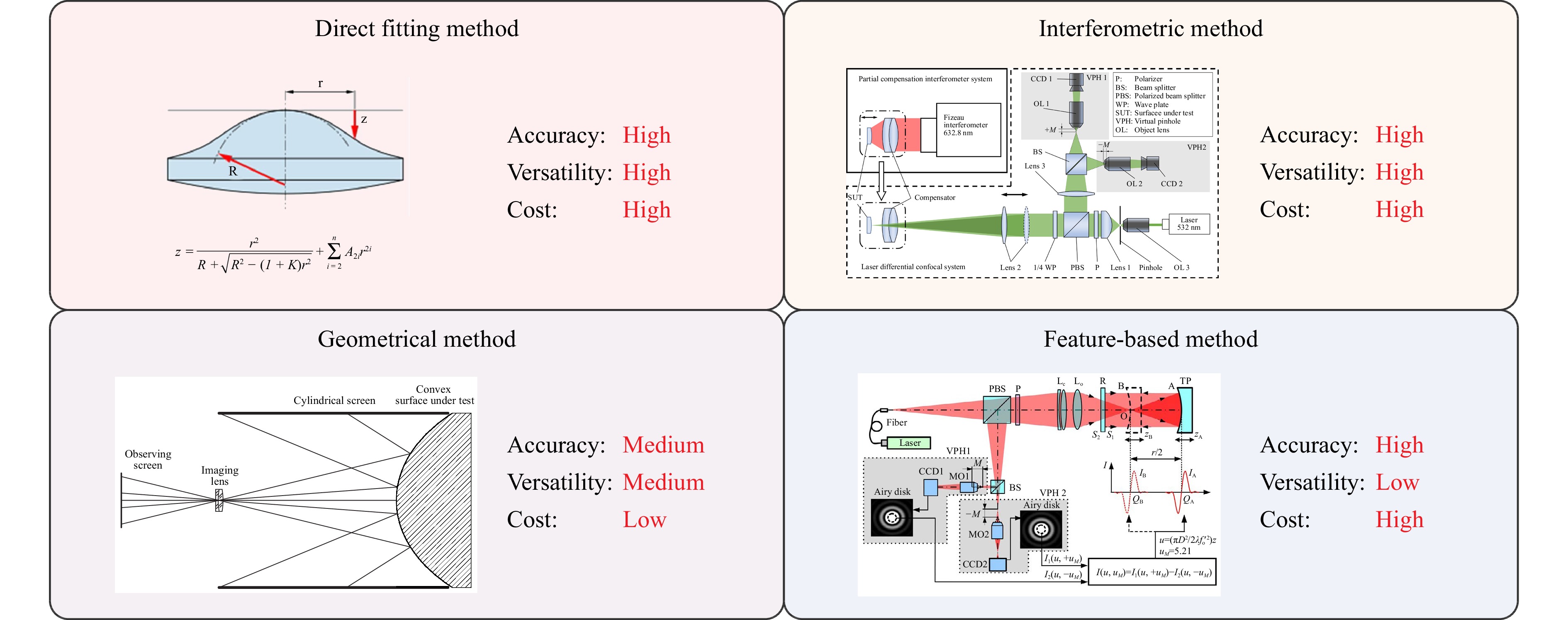
Fig. 15  Characteristics of measurement techniques for ASPs

Over the recent decades, intensive efforts have been extended to obtain highly accurate measurements. In fact, different efficient approaches have been devised for different ASUTs in various test scenarios. However, the development of advanced optics has presented new challenges. Complex boundary conditions impose strict requirements on optical shop testing. Hence, a test method that comprehensively considers high accuracy, low cost, and versatility should be devised.

National Key Research and Development Program of China (2021YFC2202404); National Natural Science Foundation of China (51735002); Strategic Priority Program of Chinese Academy of Science (XDA25020317).