


HTML
-
Lithography is fundamental to integrated circuit (IC) manufacturing; in lithography, light is passed through a patterned mask and is focused by lenses onto a resist-coated wafer. The pattern transferred on the wafer often deviates from the ideal one owing to optical proximity and thick mask effects1−3. Therefore, mask optimization, which iteratively adjusts the mask patterns to minimise the difference between the predicted wafer and target patterns, is used to compensate for these effects.
With the transition from deep ultraviolet (DUV) to extreme ultraviolet (EUV) lithography, a significantly stronger thick mask effect occurs4,5. First, because nearly all materials strongly absorb light at the 13.5 nm wavelength, EUV systems must use reflective optics with off-axis illumination. Second, the mask absorber height is several times the wavelength, which intensifies the thick mask effect. The thick mask effect in EUV lithography is typically computed using resource-intensive electromagnetic simulations to achieve the required accuracy. Consequently, implementing mask optimization in EUV lithography remains computationally prohibitive. Because EUV lithography enables continued IC shrinkage, addressing this challenge has become increasingly vital for maintaining pattern fidelity in cutting-edge IC manufacturing.
The transition to EUV also results in tighter process windows, necessitating the use of curvilinear mask patterns6−8. Unlike conventional Manhattan-style layouts with predictable right-angle features, curvilinear patterns feature arbitrary orientations and smooth curves, enabling a larger depth of focus and process window, which reflects a clear industry trend. Many compact mask models9−11 can simulate the thick mask effect, but they are difficult to apply to curvilinear patterns. Rigorous models, such as the finite-difference time-domain (FDTD) method12,13 and rigorous coupled wave analysis14, can accurately calculate the thick mask effect for curvilinear patterns but are too slow for iterative optimization. Most recently, we proposed a semi-rigorous model15 based on a modified Born series16−18 for this problem, offering a two-orders-of-magnitude speedup over the FDTD method without sacrificing accuracy.
However, this method still fails to satisfy the runtime requirements when partially coherent illumination (PCI) is considered. As shown in Fig. 1a, the illumination pupil comprises numerous source points19. Each source point requires a separate simulation using the rigorous Abbe imaging method4. In the early stages of DUV lithography, the PCI calculation can be significantly simplified by the Hopkins approximation20, which assumes that the mask diffraction is independent of the incident angle. However, this approximation is no longer feasible because of the significant thick mask effect4,21. Even for the hybrid Hopkins-Abbe method22,23, numerous near-field calculations are required. Because PCI is stochastic, the intensity I can be approached by an incoherent summation of the results from random source inputs24,25. However, many simulations are still required to achieve tolerable accuracy. Thus, improved solutions are required.
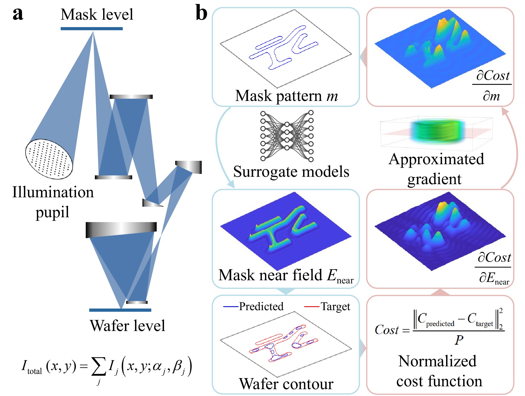
Fig. 1 EUV lithography and the proposed mask optimization framework. a Schematic overview of the lithography system. The lithography system includes four key components: the illumination pupil containing multiple source points, the mask, the projection system, and the resist-coated wafer. The total wafer intensity is obtained by summing the individual intensities $ I_{{\rm{j}}} $ from all source points. b Proposed mask optimization framework. The forward process, indicated by blue boxes, and the inverse process, marked with red boxes, form the complete optimization loop. Surrogate models generate the mask near field $ E_{{\rm{near}}} $ from the input mask pattern m. This field propagates through the projection system to produce a predicted wafer contour, which is compared against the target pattern. The deviation is averaged over the perimeter P of the target pattern. The notation $ \left\| \cdot \right\|_2^2 $ represents the square of the $ {l_2} $-norm. The partial derivative of the cost function with respect to the mask near field is computed through the chain rule. Finally, the approximated gradient of the mask pattern is calculated for mask modification.
Motivated by the fast inference capability of deep learning models, various architectures have been explored as surrogate models for EUV mask modelling26. Representative examples include U-Net27, generative adversarial networks28, and physics-informed neural networks29. To date, no reports have been published on surrogate models that simultaneously consider both PCI and curvilinear patterns, both of which are crucial for practical EUV mask optimization.
In addition to forward modelling, deep learning has been applied to end-to-end inverse optimization30,31. However, the training data for these end-to-end methods rely on iterative methods, among which heuristic methods are inefficient32,33. Furthermore, the outputs of end-to-end methods are not guaranteed to be optimal and typically require additional fine-tuning via gradient-based methods26, making gradient computation indispensable. The existing gradient computation for the EUV mask model relies on the adjoint method34, which requires storage of the 3D field within the mask. This leads to excessive memory consumption, making mask optimization, and consequently full-chip optimization, impractical when PCI is considered. Gradient computation for mask models poses significant additional challenges beyond forward modelling. As shown in Fig. 1b, gradient computation involves the partial derivative of the cost function with respect to the mask near field, which is an exceedingly more complex input than the simple plane-wave incidence used in forward modelling.
The model complexity introduced by curvilinear patterns, heavy computational cost induced by PCI, and large memory requirements from gradient calculations form a compounded problem, which makes EUV mask optimization challenging, particularly at the full-chip scale35. Although a single pattern is manageable, achieving sub-nanometre accuracy across a full millimetre-scale chip within a reasonable computation time is extremely difficult.
In this paper, we propose the first publicly described full-chip EUV mask optimization framework that simultaneously considers accurate thick mask modelling, curvilinear patterns, and PCI. As shown in Fig. 1b, it consists of deep-learning-enabled surrogate models for forward modelling and a mask gradient calculation for inverse optimization. Trained by high-accuracy data generated by the fast EUV mask model based on the modified Born series, surrogate models are used to predict the mask near fields for various source points. They achieve excellent consistency with the reference model while being approximately two orders of magnitude faster. We also propose an approximated gradient to support gradient-based optimization. We validated the proposed framework using classical logic and BigMaC patterns36 and demonstrated its accuracy and reliability. Furthermore, we present a large-scale mask optimization example and provide a runtime estimation for full-chip applications. The proposed framework enables a feasible full-chip EUV mask optimization, which has been previously computationally intractable for practical implementation. It has the potential to significantly advance computational lithography and IC fabrication.
-
The EUV mask consists of an absorber and multilayer, as shown in Fig. 2a. The multilayer and thickness of the absorber are fixed, and the absorber pattern is subjected to variations during mask optimization. The incident field is a set of plane waves determined by the PCI, each consisting of three complex-valued two-dimensional (2D) arrays corresponding to the x-, y-, and z-polarizations. The inputs of EUV near-field calculations include the wave vector $ \vec{r} $, field vector $ {{\vec{E}}_{\rm {in}}} $, and mask pattern. The output is a mask near field containing three complex-valued 2D arrays.
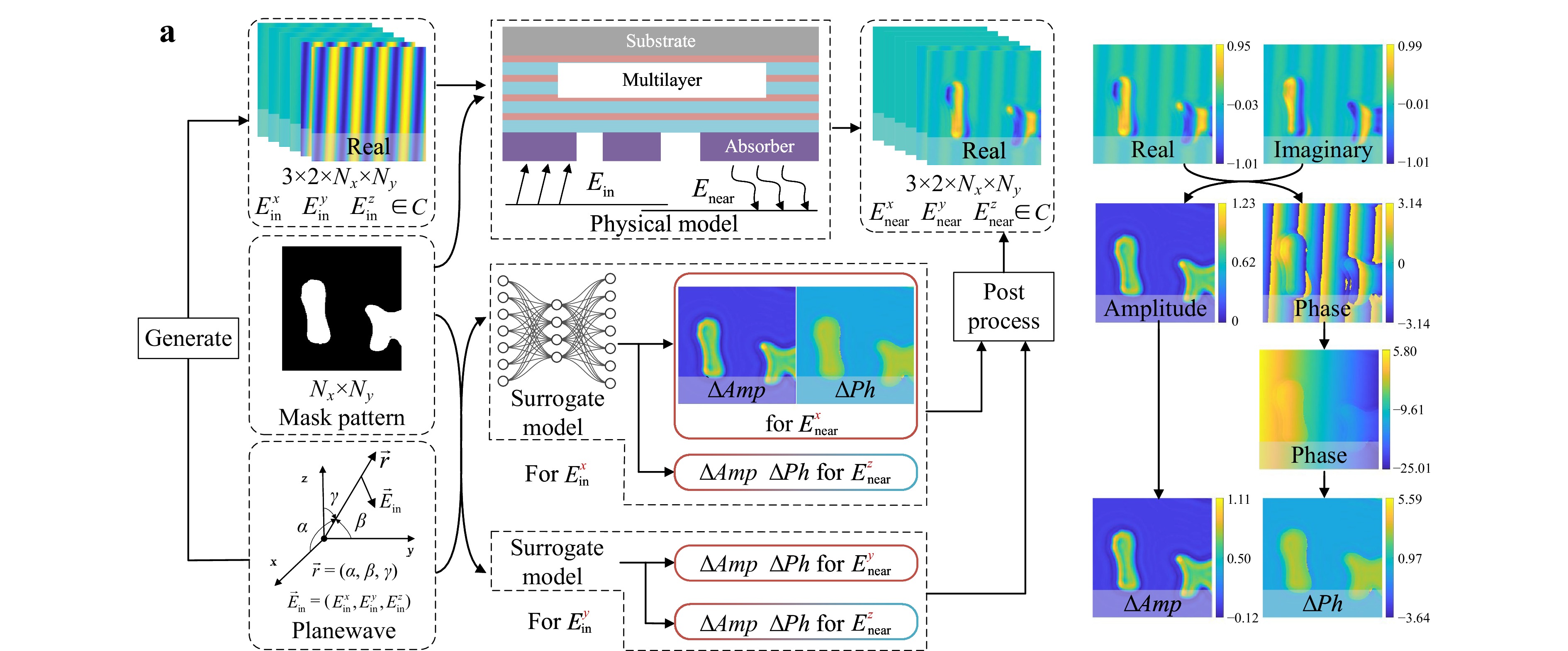
Fig. 2 Schematic diagram of the reference EUV mask model and surrogate models. a Comparison between the reference and surrogate models. The incident field for the reference model is generated from the plane wave parameters. The incident field and mask pattern are used as the input, and the near field can be obtained from the physical model. The surrogate model uses plane wave parameters as input instead of the incident field. The prediction, including the amplitude perturbation $ \Delta Amp $ and phase perturbation $ \Delta Ph $, can be further processed to get the final result. Two surrogate models exist for the x- and y-polarized incident fields, respectively. b Processing flow of the field representation. The complex field is stored as the combination of real and imaginary parts in computers. Subsequently, the field is represented by the amplitude and phase. The amplitude perturbation $ \Delta Amp $ is obtained by subtracting the reference amplitude, whereas the phase perturbation $ \Delta Ph $ is unwrapped before the subtraction.
The mask shadowing effect is the key phenomenon to capture. In addition, the interference between adjacent features must also be considered. The diffraction of the absorber is governed by both the polarization and orientation of its features37. With the maturation and application of curvilinear masks8,38, the shadowing effect of the EUV mask becomes increasingly convoluted. The reflection from the multilayer is also dependent on the polarization and incident angle. Thus, the effects of the mask pattern, incident angle, and polarization on the near field are intricate and multifaceted.
Based on these considerations, an accurate EUV mask model based on the structure decomposition method was adopted15. The modified Born series (MBS) method16−18 and transfer matrix method39 were used to simulate diffraction in the absorber layer and reflection in the multilayer, respectively. This mask model served as the reference model in this study and provided training data for the surrogate models.
Three primary considerations are essential for constructing the surrogate models. First, the near field is complex-valued. Although complex-valued models are available40, they suffer from limited research, fewer implementations, and less community support compared with their real-valued counterparts. In most studies, a field is represented by its real and imaginary parts27,41,42. This representation is straightforward in algebra but not physically intuitive43. Instead, we use the amplitude and phase to represent the near field.
Second, because of the dependence of the reflection coefficients of the multilayer on the incident angle44, slight amplitude fluctuations and phase shifts occur at different incident angles, even in the absence of any pattern. To reduce the complexity of the surrogate models further, we remove the fluctuations and shifts in data preparation. The processing flow is shown in Fig. 2b. The reference amplitudes and phases are obtained in advance from simulations without patterns using the reference model. The reference amplitude is subtracted from the actual amplitude. The phase is unwrapped to eliminate sudden discontinuities from $ -{\text{π}}$ to π. The unwrapped reference phase is subtracted from the unwrapped phase. Consequently, a model is required to predict amplitude perturbation $ \Delta Amp $ and phase perturbation $ \Delta Ph $.
If the near field is represented in terms of real and imaginary parts, periodic stripes will occur on both the background and pattern features owing to oblique incidence, as shown at the top of Fig. 2b. Consequently, even stripes on the same pattern feature will differ depending on their position, which is unrelated to the mask shadowing effect and will be challenging for the surrogate models to mimic. Instead, the proposed perturbation-based representation is space-invariant and free of redundancy, directly capturing the physical essence of the problem, thereby reducing both model complexity and inference time. As shown in the Supplementary Information, our model maintains a constant of 16 channels in all convolutional layers, in contrast to typical designs that start with 32 channels and increase them exponentially across the layers28,41.
Third, the incident plane wave comprises fields with different polarizations that interact differently with the pattern, as mentioned earlier. The polarization conversion during diffraction caused by an absorber increases the complexity of this problem. Therefore, we use different models for each incident polarization, with each model predicting the corresponding perturbations. As shown in Fig. 2a, the model for $ E_{\rm{in}}^{x} $ predicts $ \Delta Amp $ and $ \Delta Ph $ of the $ E_{\rm{near}}^{x} $ as well as $ E_{\rm{near}}^{\textit{z}} $. The $ E_{\rm{near}}^{{y}} $ contribution by $ E_{\rm{in}}^{{x}} $ is ignored because of its low energy. Based on the linearity of Maxwell's equations, the near fields from different incident polarizations can be summed to obtain the near field. Details of the model are provided in the Supplementary Information.
-
The gradient, which is the derivative of the cost function with respect to the mask pattern, is essential for efficient mask optimization. Other components of lithography models are differentiable45,46. This section focuses on the gradient calculation of mask models. The gradient calculation is inherently supported by mainstream artificial intelligence (AI) frameworks. However, surrogate models are trained for outputs rather than for the partial derivative of the outputs with respect to the inputs, implying that the gradients generated by the surrogate models are questionable. Although this problem can be alleviated by employing differentiation-friendly operations inside surrogate models, this may compromise the prediction accuracy at a given level of model complexity.
By resorting to the physical model, we propose an approximate gradient for the surrogate models, as depicted in Fig. 3. The adjoint method computes the gradient of a cost function with respect to design parameters by applying a chain rule and solving the corresponding adjoint simulation. This avoids explicit differentiation of the system state by exploiting the optical reciprocity between the sources and fields34,47. In mask optimization, the incident field of the adjoint simulation $ E_{\rm{in}}^{\rm{adj}} $ is defined as the partial derivative of the cost function with respect to the mask near field, thereby enabling gradient computation with respect to the refractive index. A linear function f representing the postprocessing operations34, is applied to obtain the gradient with respect to the mask pattern.
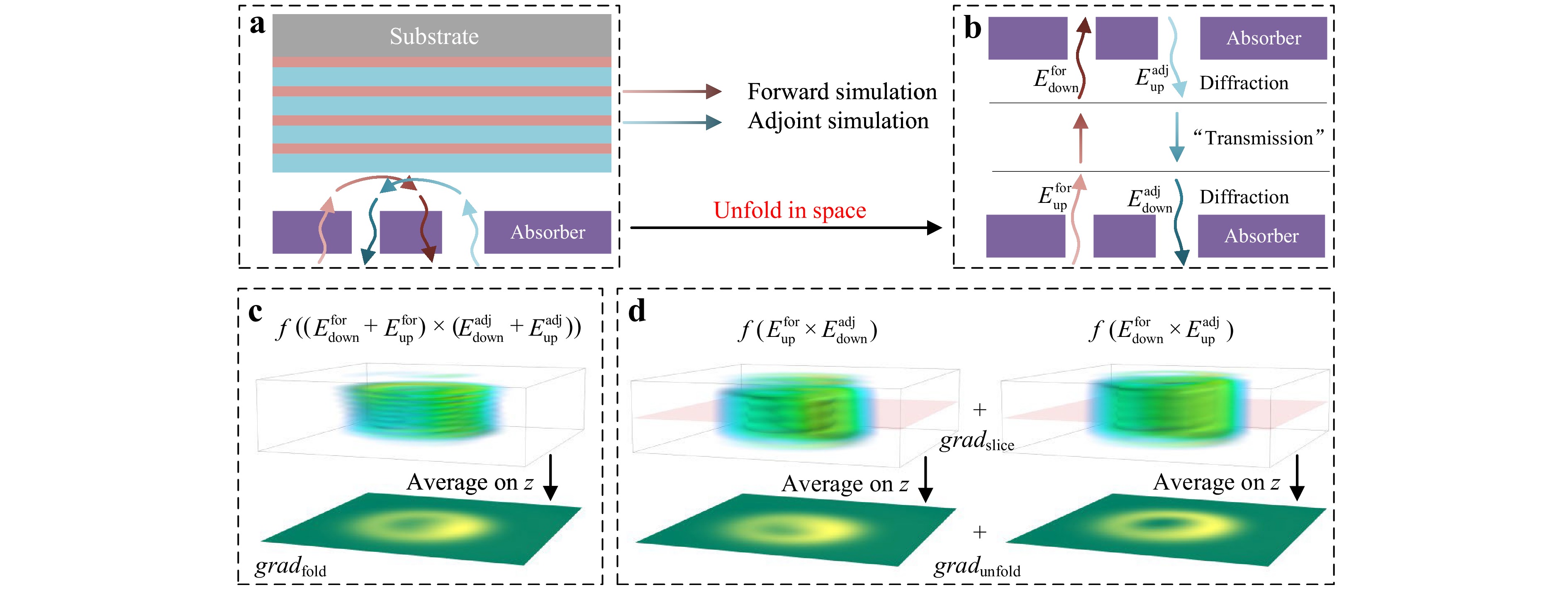
Fig. 3 Gradient calculation for the surrogate model. a Schematic of gradient computation for $ {grad_{\rm{fold}}} $. Forward and adjoint simulations are required to obtain the gradient. The green and red arrows with a gradual colour shift are used to represent the light trace in forward and adjoint simulations, respectively. b Schematic of gradient computation for $ {grad_{\rm{unfold}}} $ and $ {grad_{\rm{slice}}} $. Physically, the downward and upward diffraction processes are overlapped in space, whereas they are separate and unfolded in simulations. c Computational process of $ {grad_{\rm{fold}}} $. The fields in the forward and adjoint simulations are added, multiplied, and averaged along the z-axis to obtain the gradient. The function f is linear and contains post-processing operations34. The 3D plot of the gradient shows significant fluctuations along the z-axis. The symbols for the corresponding quantities are labelled above the plot. d Computational process of $ {grad_{\rm{unfold}}} $ and $ {grad_{\rm{slice}}} $. The unfolding scheme circumvents the interference of fields from downward and upward diffraction, which significantly alleviates the fluctuations of the gradient. Furthermore, the slicing scheme skips the averaging operation, enabling its application to surrogate models.
The optimization variable is the mask pattern, which defines the absorber layer. Therefore, the field discussed below focuses on the absorber region, whereas the field inside the fixed multilayer is ignored. In the reference model, the gradient calculation can be expressed as
$$ grad = \frac{{\partial {Cost}}}{{\partial m}} = f\left( {{E^{{\rm{for}}}} \times {E^{{\rm{adj}}}}} \right) $$ (1) where $ {E^{\rm{for}}} $ and $ {E^{\rm{adj}}} $ are the fields in the forward and adjoint simulations, respectively. Typically, near-field calculations involve downward diffraction through the absorber, reflection from the multilayer, and subsequent upward diffraction through the absorber, as shown in Fig. 3a. Owing to the reflection of the multilayer, the fields from the downward and upward diffractions coincide in space.
$$ E = {E_{{\rm{down}}}} + {E_{{\rm{up}}}} $$ (2) In addition, all fields are 3D arrays, whereas the design variable is a 2D array. Substituting Eq. 2 into Eq. 1 and averaging along the z-axis yields,
$$ grad_{{\rm{fold}}} = {{\rm{avg}}_{\textit{z}}}\left( {f\left( {\left( {E_{{\rm{down}}}^{{\rm{for}}} + E_{{\rm{up}}}^{{\rm{for}}}} \right) \times \left( {E_{{\rm{down}}}^{{\rm{adj}}} + E_{{\rm{up}}}^{{\rm{adj}}}} \right)} \right)} \right) $$ (3) The gradient calculation in Eq. 3 cannot be applied to the surrogate models because of the lack of these 3D field arrays. The proposed surrogate models provide only 2D arrays that represent the near field at a specified height. Note that an averaging operation exists. If the slices of the gradient $ {grad_{\rm{fold}}} $ before averaging are similar, then the gradient can be approximated using an arbitrary slice. However, as shown in Fig. 3c, a strong fluctuation occurs along the z-axis owing to the interference between $ {E_{\rm{down}}} $ and $ {E_{\rm{up}}} $. An unfolded scheme is proposed to alleviate this fluctuation, as shown in Fig. 3b. Although $ {E_{\rm{down}}} $ and $ {E_{\rm{up}}} $ physically coincide in space, they can be separated by considering reflection operations as a type of transmission in the computation. In other words, these two fields are obtained through different simulations, and they need not overlap in the computation. Eq. 3 can be rewritten as
$$ gra{d_{{\rm{unfold}}}} = {{\rm{avg}}_{\textit{z}}}\left( {f\left( {E_{{\rm{down}}}^{{\rm{for}}} \times E_{{\rm{up}}}^{{\rm{adj}}}} \right) + f\left( {E_{{\rm{up}}}^{{\rm{for}}} \times E_{{\rm{down}}}^{{\rm{adj}}}} \right)} \right) $$ (4) The two terms on the right-hand side of Eq. 4 are shown in Fig. 3d. The fluctuation is significantly suppressed. Consequently, a single slice is sufficient to approximate the gradient rather than requiring the entire 3D field array. Although this method does not eliminate fluctuations entirely, it remains viable and effective, as demonstrated in the following examples.
Herein, we present a detailed implementation of the slice scheme using surrogate models.
$$ gra{d_{{\rm{slice}}}} = f\left( {E_{{\rm{down}}}^{{\rm{for - bpm}}} \times E_{{\rm{up}}}^{{\rm{adj - bpm}}}} \right) + f\left( {{E_{{\rm{near}}}} \times E_{{\rm{in}}}^{{\rm{adj}}}} \right) $$ (5) where $ {E_{\rm{down}}^{\rm{for}-{\rm{bpm}}}} $ and $ {E_{\rm{up}}^{\rm{adj}-{\rm{bpm}}}} $ are the corresponding fields at the same slice obtained using the beam propagation method (BPM). The BPM is a scalar electric field solver suitable for weak scattering problems48. The details of the BPM unit are provided in the Supplementary Information. Note that the first term on the right-hand side of Eq. 5 is based on scalar simulations. This is a compromise, because vector simulations are computationally more expensive. Operations such as the approximation and averaging discussed here are conducted solely within the gradient calculation workflow and do not affect the accuracy of the forward simulation. A detailed investigation of the accuracy of the surrogate model and approximated gradient is provided in the Supplementary Information.
-
An example of EUV mask optimization is shown in Fig. 4a. The target pattern is a BigMaC pattern with a minimum wafer CD of 19.41 nm. The curvilinear binary mask is obtained using the level-set method49, which inherently supports curvilinear mask evolution50. Mask optimization involves three stages characterised by varying the numbers of source points $ {{N}}_{\rm{source}} $. In the first stage, the mask is optimised under only one source point in the middle of the illumination pupil. In the second and third stages, the mask is optimised under 42 and 332 source points, respectively.
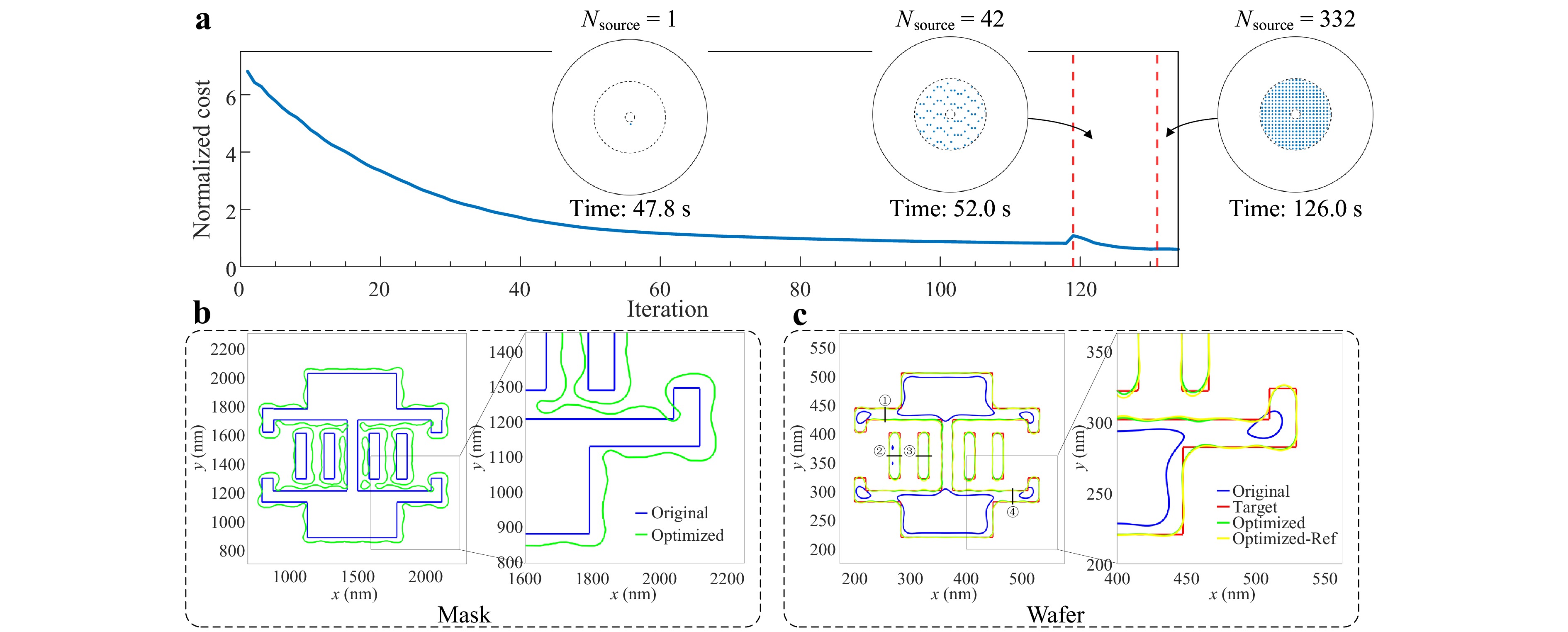
Fig. 4 Mask optimization example on a BigMaC pattern with the critical dimension of 19.41 nm. a Convergence of the normalized cost during the optimization. The optimization consists of three stages, each characterized by a different number of source points $ {{N}}_{\rm{source}} $. b Comparison between the original and optimised mask pattern contours. The right-hand figure is a magnified view. c Comparison between the original, target, optimised, and verified wafer pattern contours. The verified wafer contour is obtained using the reference model. The right figure is a magnified view. The numbers and black lines in the figure mark the locations of critical dimension measurement.
The target pattern serves as the initial mask in the first stage. The subsequent stages inherit the optimised mask pattern from their immediate predecessor as the initial configuration. The first stage conducts coarse optimization using a single source point, effectively reducing the overall runtime by requiring fewer iterations in later stages, where each iteration is more computationally expensive. A pronounced surge in the convergence curve of the normalised cost function is observed at the first-to-second stage transition, resulting from an abrupt increase in source points. This surge demonstrates the necessity of considering PCI in mask optimization. Conversely, a smaller variation occurs between the second and third stages, indicating that mask optimization with 42 source points provides a sufficient solution. However, for higher precision, optimization with additional source points is recommended.
The cost function decreases consistently and reaches the optimised state after 135 iterations. The mask patterns before and after optimization are shown in Fig. 4b. The mask is extended to compensate for the thick mask effect, and some topology changes occur at locations with dense patterns. Although the absence of mask rule checks results in some narrow spacings, it also highlights the robustness of the model in complex scenarios. Mask rule checking can be incorporated in future research. The corresponding wafer patterns are shown in Fig. 4c. The original wafer pattern undergoes significant distortion, whereas the optimised wafer contour closely matches the target contour. In addition, the optimised wafer contour from the reference model aligns closely with that of the surrogate model. We also performed multiple CD measurements at the locations shown in Fig. 4c. A comparison of these results is presented in Table 1. The relative errors are below 3.5%, confirming the accuracy of the surrogate model.
Locations ① ② ③ ④ Surrogate CD 20.35 19.14 19.33 19.32 Reference CD 20.66 19.53 19.98 19.15 Relative Error −1.48% −2.04% −3.22% 0.89% Table 1. Critical dimension comparison. (nm)
The key driving force behind the adoption of surrogate models is their impressive speed advantage over reference models. With a GPU of NVIDIA A100, the combined inference time for the two surrogate models is approximately 3.4 ms, whereas the reference model takes 892.3 ms to calculate the same mask. The surrogate models are two orders of magnitude faster than the reference model. The total runtime for this example, covering an area of 0.53 μm2 (0.73 μm × 0.73 μm) at the wafer scale, is approximately 225.8 s. The total time required to prepare the surrogate models, including data generation, preprocessing, and training, should be within 12 h using two A100 GPUs, although these are not precisely measured.
An example of a large-scale mask optimization is presented in Fig. 5. The entire pattern consists of repeating classical logic patterns rotated from 0° to 360° while the illumination remains fixed. The optimised mask pattern is cropped and rotated to visualise its response under different incident directions, as shown in the Supplementary Information. Part of the result with an approximate 45° rotation is validated by the reference model, as shown in Fig. 5b, demonstrating excellent consistency. Notably, the training data for the surrogate models contained no intentional rotations, highlighting their strong generalisability.
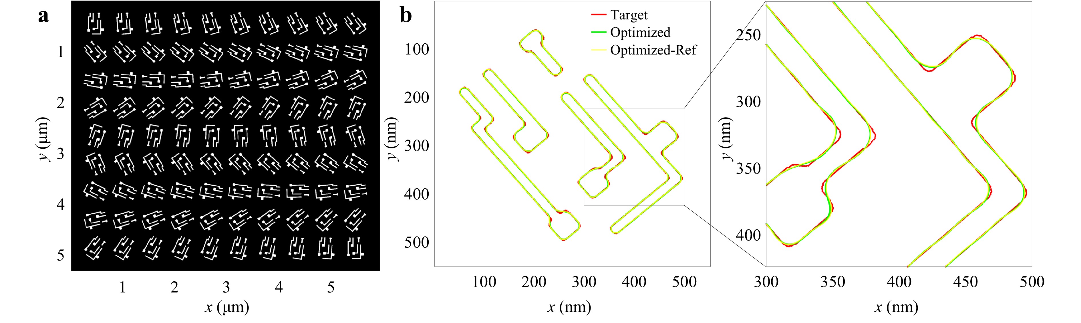
Fig. 5 Example of large-scale mask optimization. a Target pattern of the mask optimization on wafer scale. It consists of repeating classical logic patterns rotated from 0° to 360°. b Comparison between the target, optimised, and verified wafer pattern contours. The verified wafer contour is obtained using the reference model.
The third stage shown in Fig. 4a is skipped in this example. The cost convergence is shown in Fig. S5. The target pattern of this example covers an area of 31.4 μm2 (5.90 μm × 5.31 μm) at the wafer scale. The runtime is approximately 59.7 min using the same hardware as mentioned above. Assuming linear scalability and using 1,000 GPUs, mask optimization for a 1 $ {{\rm{mm}}^2} $ area at the wafer scale, which is 31,847 times larger than the demonstrated area, can be completed in $ 31,847\, \times \,59.7\, \div \,60\, \div\, 1,000 \,\approx \,31.7 $ h. This demonstrates the potential of full-chip mask optimization.
The mask optimization examples in the main text do not intentionally include sub-resolution assist features (SRAFs), which may lead to a suboptimal through-focus performance. However, this is beyond the scope of this paper. If included, SRAFs can be seamlessly co-optimised within the same process at no extra computational cost. Additionally, the Supplementary Information includes a mask optimization example with inserted SRAFs under Y-dipole illumination, which further validates the flexibility of our framework.
-
Highly efficient and accurate EUV mask optimization has been demonstrated in this paper, distinguished by ultrafast surrogate models and an approximated gradient. The surrogate models are two orders of magnitude faster than the reference model and up to four orders of magnitude faster than the FDTD method15. The approximated gradient bypasses the direct gradient computation in the surrogate models, thereby avoiding the potential accuracy degradation of the forward simulations. These examples validate the accuracy of the surrogate models and effectiveness of the approximated gradient. Because runtime is a primary adoption barrier5,50, the demonstrated speedup is crucial for advancing computational lithography. The proposed framework expands the applications of computational lithography and supports the development of next-generation ICs. Furthermore, the core methodology presented in this paper can be applied to other fields related to large-scale simulations and optimization, including metasurfaces51−53 and photonic circuits54−56.
Although numerous EUV mask models exist, they typically address the features outlined in the introduction in isolation or in partial combinations. Crucially, these features are not simply additive; they involve complex coupling that our framework is specifically designed to handle. Consequently, methods with fundamentally different scopes are not directly comparable. This paper introduces the first full-chip EUV mask optimization framework that simultaneously considers accurate thick mask modelling, curvilinear patterns, and PCI. Consequently, no direct predecessor exists for a performance comparison. The closest existing work capable of high-accuracy EUV mask optimization simulates the EUV mask using the modified Born series15,34, which calculates the interaction between the incident field and the EUV mask using 3D convolution with the Green’s function. In contrast, the proposed framework utilizes 2D convolution in deep learning. The fundamental transition from 3D to 2D operations results in significant advantages in terms of time consumption, memory requirements, and scalability. The existing method requires approximately 71 h for the same optimization task, as shown in Fig. 4, assuming a linear relationship between runtime and the number of source points. In addition, the existing method stores large 3D arrays for gradient calculation, requiring 15 times more memory than the proposed method. The advantages of the proposed framework are amplified for large-scale applications, significantly affecting its feasibility and scalability. In addition, deep learning models are inherently well-suited for parallelization and large-scale applications.
Recently, the emergence of large language models has led to the proliferation of GPU-based servers and computing centres, laying the foundation for large-scale industrial applications of the proposed framework. Not only is the existing hardware support mature but the algorithm transition is also smooth. The most common mask model for DUV lithography is based on convolution operations, which convolve layout properties, such as the polygon area and edges, with calibrated filters11,57. Instead of highly skilled engineers designing the convolutions manually, the filters in the proposed framework can be trained automatically, enabling them to handle more sophisticated scenarios. Each surrogate model contains approximately 60,000 parameters. Although the predictions from the surrogate models may contain some errors compared with those from the rigorous simulations, the average of these predictions, as required by PCI, would be close to the rigorous one. In other words, the average of the surrogate model predictions is expected to be robust and reliable.
The accuracy of the reference model is comparable to that of the FDTD method15, providing a reliable foundation for the model. Moreover, the framework is not constrained to a specific reference model. Any EUV mask model that can generate accurate near fields within a practical time can be applied. The other components of the lithography model, including the projection and resist models, are widely used and are sufficient for this proof-of-concept study, which focuses primarily on the mask model.
A framework combining surrogate models with gradient-based optimization is well-established in applications such as metasurfaces58,59, where it typically maps a few unit-cell parameters to a few output values or spectral responses. In contrast, this paper addresses a 2D-to-2D problem. High dimensionality and complexity render direct gradient computation impractical. The proposed gradient calculation method enables the application of this established paradigm in our context for the first time.
As demonstrated above, the proposed method can effectively address large-scale EUV mask optimization with acceptable time consumption. Certain improvements can be implemented, such as adding a surrogate mask model for the z-polarised incident field, training the models for a full-illumination pupil, and using high-NA EUV lithography. Future research may extend this work to source-mask optimization. The proposed framework may also be applicable to DUV lithography using the FDTD method as the reference model. Furthermore, the gradient calculation is independent of the surrogate models, which allows higher precision to be achieved with alternative deep learning architectures. More efficient optimization algorithms can be applied to reduce runtime.
-
Lithography model The lithography model often comprises four main components: PCI, mask model, projection model, and resist model. In this work, the PCI was annular, with a partial coherence factor of 0.6 for the outer edge and 0.06 for the inner edge. The number of source points corresponded to 332. The mask model employed a 50 nm-thick TaN absorber with a complex refractive index of $ N = 0.938499+0.037757{{i}} $. The near field was sampled at a plane located 13.5 nm above the absorber. The multilayer containing intermixing layers was adopted44. The vector-projection model was used to calculate the field on the wafer plane using a mask near field60,61. The numerical aperture and demagnification of the simulated aberration-free projection system were 0.33 and 4, respectively. Defocus was not considered in the demonstrated examples but can be incorporated within the system. A sigmoid function was adapted as the resist model with a steepness of 80 and a threshold of 0.4. Other resist models with higher accuracy can be applied62,63 provided that they are differentiable.
Mask optimization Mask optimization was performed iteratively using the steepest descent method. The maximum step size was determined using the Courant-Friedrichs-Lewy (CFL) condition using a CFL factor of 4. The actual step sizes were determined using Brent’s method64 with five evaluation. Linearized gradient34 was used in the first stage of optimization, whereas a normal gradient was applied in the other stages.
While evanescent waves in the near field influence gradient calculations, they are filtered out by the projection lens and do not contribute to the aerial image, which can potentially introduce instability in mask optimization. To suppress these instabilities, we employed two regularisation techniques: curvature motion and reinitialization. During level-set evolution65,66, an additional motion driven by the mean curvature of the pattern contour was applied to reduce the complexity of the pattern. The strength factors of the curvature motion were 0.012 and 0.008 for examples in Figs. 4 and 5, respectively. The implicit level-set function was reinitialized every four iterations.
In the first stage of the mask optimization, convergence criteria consisted of a maximum iteration limit of 120 and a cost function threshold of 0.5. In the second stage, the maximum iteration limit and cost function threshold were changed to 50 and 0.2, respectively. Additionally, the optimization was terminated when the cost function change remained below 0.02 for four consecutive iterations. In the final stage, the maximum iteration limit was reduced to 20 while maintaining all other convergence criteria from the second stage.
Surrogate models The mask pattern varied in size, whereas the surrogate models received input with a fixed shape. Hence, the surrogate models used 256 × 256 pattern tiles cropped from the mask pattern with a 40-pixel overlap. The outputs were then merged and the outermost 20 pixels of each output were discarded. The surrogate models were based on a tuneable U-net67, which consisted of one encoder for the pattern, one fully connected network for the plane wave parameters, and one decoder for the outputs. The output of the fully connected network was reshaped and directly appended to the encoder output, which served as part of the input to the decoder. More details regarding the data preparation, model configuration, and training are provided in the Supplementary Information.
-
This research was supported by the National Natural Science Foundation of China (52130504 and 52305577), Major Program (JD) of Hubei Province (2025BEA006), Huazhong University of Science and Technology's Major Science and Technology Innovation Program (2024ZDKJCX09), Innovation Project of Optics Valley Laboratory (OVL2023PY003), Postdoctoral Fellowship Program (Grade B) of China Postdoctoral Science Foundation (GZB20230244), Fellowship from the China Postdoctoral Science Foundation (2024M750995), and Postdoctor Project of Hubei Province (2024HBBHCXB011). The authors are grateful for the technical support provided by the Experiment Centre for Advanced Manufacturing and Technology at the School of Mechanical Science and Engineering of HUST. The computations were completed on the HPC Platform of Huazhong University of Science and Technology.

 DownLoad: