Breaking the speed limitation of wavemeter through spectra-space-time mapping

Accurate high-speed measurements of wavelength are fundamental to environmental monitoring¹, biomedical analysis², and material characterization³. Conventional spectrometers disperse light to different spatial locations using dispersion elements such as gratings. However, their resolutions are limited by their spatial size⁴. Recent studies have shown that a disordered scattering medium such as a multimode fiber (MMF) can generate a wavelength-dependent speckle pattern, which is used to reconstruct the spectrum of incident light^5-6. MMF-based spectrometers can provide a high spectral resolution and broad operation bandwidth in a compact structure.

One of the current objectives of spectroscopy research is to improve the measurement speed for fast and non-repetitive events such as chemical reactions, ultrashort pulses, laser mode-locking dynamics, and spatiotemporal solitons. However, most speckle-based spectrometers use imaging sensors based on charge-coupled devices (CCD) or complementary metal–oxide–semiconductor (CMOS) technology to record speckle patterns, which are widely known for their slow measurement rates, usually between 10 Hz and 10 kHz. Therefore, the measurement speeds of current speckle spectrometers are constrained by cameras, which limits their applications. Although ultrafast cameras can achieve faster measurement rates, they are expensive and significantly increase the system costs. Another solution is to replace the imaging sensor with spatial-to-temporal mapping technology, but it also requires complex and costly optical systems⁷.

A transmission matrix is typically used to reconstruct a spectrum^8-9. The spectral resolution is determined by the minimal change in wavelength that generates an uncorrelated speckle pattern. Many reconstruction algorithms have been proposed to improve the resolution and operating bandwidth. In addition, multivariate analysis methods such as principal component analysis have been used to overcome the resolution limitation of correlations between speckle patterns¹⁰. However, principal component analysis only allows for a limited operating range and low processing speed^11-12. Alternatively, compressed sensing has been applied to increase the operating bandwidth when reconstructing sparse spectra¹³ and to increase the measurement rate without reducing resolution. However, compressed sensing is not suitable for analyzing data containing environmental noise. Recently, deep learning has attracted considerable attention. A deep-learning system can automatically extract features from data at multiple levels of abstraction, allowing the direct learning of complex functions that map the spectrum to the speckle pattern. High-accuracy estimation can be achieved over a broad operating range with robustness to instrumental and environmental noise^14-15. Combining convolutional neural networks and speckle patterns obtained using cameras enables highly accurate wavelength measurements.

This paper presents and validates a pioneering approach to overcome this speed limit. We propose a low-cost, high-speed wavemeter based on an MMF and multicore fiber (MCF) structure. MCFs are commonly used in space-division multiplexing systems. Owing to the similarity in cladding diameters between MCF and MMF, they have been fused for spatial dimension multiplexing¹⁶. The MMF generates a wavelength-dependent speckle pattern, which is spectral-to-spatial mapping. We then used a seven-core MCF to sample the speckle pattern, replacing the common camera to avoid frame rate limitations, thereby providing spatial-to-temporal mapping, as illustrated in Fig. 1. The light pulses in the MCF are then separated by a set of delay lines and detected using a single photodetector. Our frequency-space-time mapping-based wavemeter has an all-fiber structure that considerably increases the measurement speed at a low cost. A multilayer perceptron (MLP) is employed to estimate the wavelength from the pulse sequences of the speckle patterns. Sampling the speckle patterns of the MMF using the MCF reduces the amount of input data efficiently, allowing for a simple network structure to perform the wavemeter function, thereby reducing system complexity. The feasibility and effectiveness of the proposed high-speed wavelength-estimation method are experimentally verified. We demonstrate a wavemeter with a 100 MHz measurement rate and 2.7 pm precision.

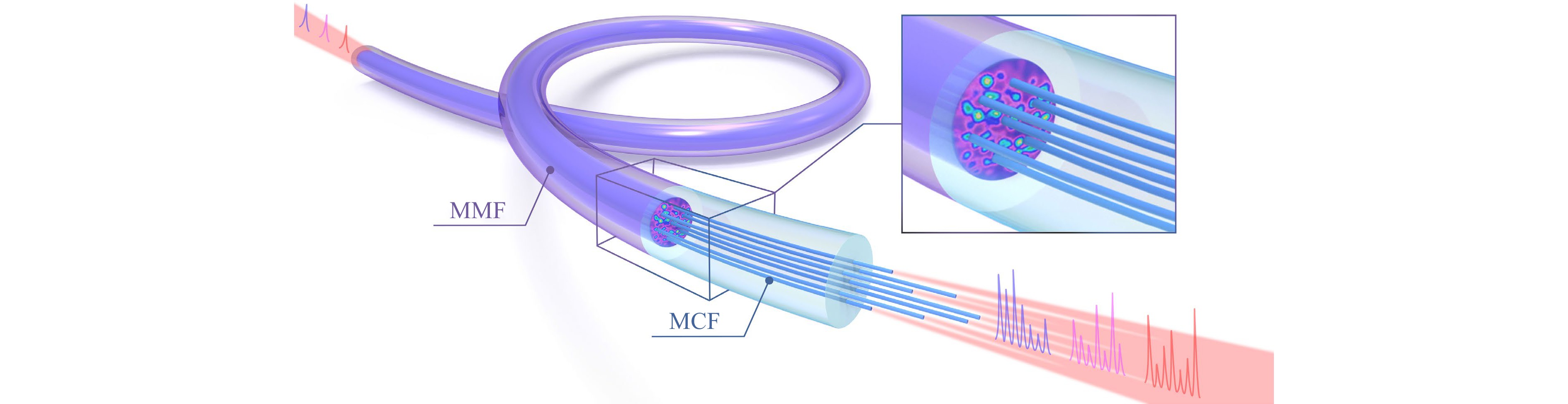
Fig. 1  Evolution of light pulse in MMF and MCF. The input pulse is mapped into a speckle pattern through the MMF. Then, the MCF samples the output pattern into a pulse sequence. The seven cores of the MCF are extended in different lengths to avoid overlapping.

The remainder of this paper is organized as follows: Section 2 describes the experimental apparatus and introduce the principles of data acquisition and MLP. Experimental results and analyses are presented in Section 3. The influence of the number and position of MCF cores on accuracy is also discussed in this section. Finally, the conclusions are presented in Section 4.

The experimental setup for the proposed MMF–MCF wavemeter is shown in Fig. 2. A tunable laser (CoBrite ID Photonics DX4) was used to generate the monochromatic light. An in-phase/quadrature (I/Q) modulator was employed to change the wavelength of incident light and convert it into pulsed light. Single-sideband modulation (SSB) shifts the frequency and controls the input wavelength. The I/Q modulator consists of two Mach–Zehnder intensity modulators with a π/2 phase shifter between the two arms. When the two arms of the I/Q modulator are loaded with the sine and cosine signals of frequency ${f_m}$, the light frequency shifts to ${f_0} + {f_m}$ , where ${f_0}$ is the frequency of the incident light (detailed principles are provided in the supplemental document)¹⁷. The I/Q modulator was controlled using an arbitrary waveform generator (Keysight M8196A), which generated high-speed light pulses with controlled wavelength variation signals. The detailed parameter settings are described in Section 2.2. The output light was amplified using an erbium-doped optical fiber amplifier, which was used to compensate for the loss in the I/Q modulator. These devices are used to rapidly adjust the wavelength of the incident light to simulate high-speed measurement scenarios, which are not required in real measurement systems. We employed a fiber polariser (FP) to maintain a consistent input polarization state into the MMF to mitigate slight fluctuations in the laser and fibers. The polarization state variations before the FP only affect the MMF output speckle’s total power without altering the peak power ratios of the pulse sequences. A fiber polarization controller (FPC) cooperated with the FP to minimize power loss.

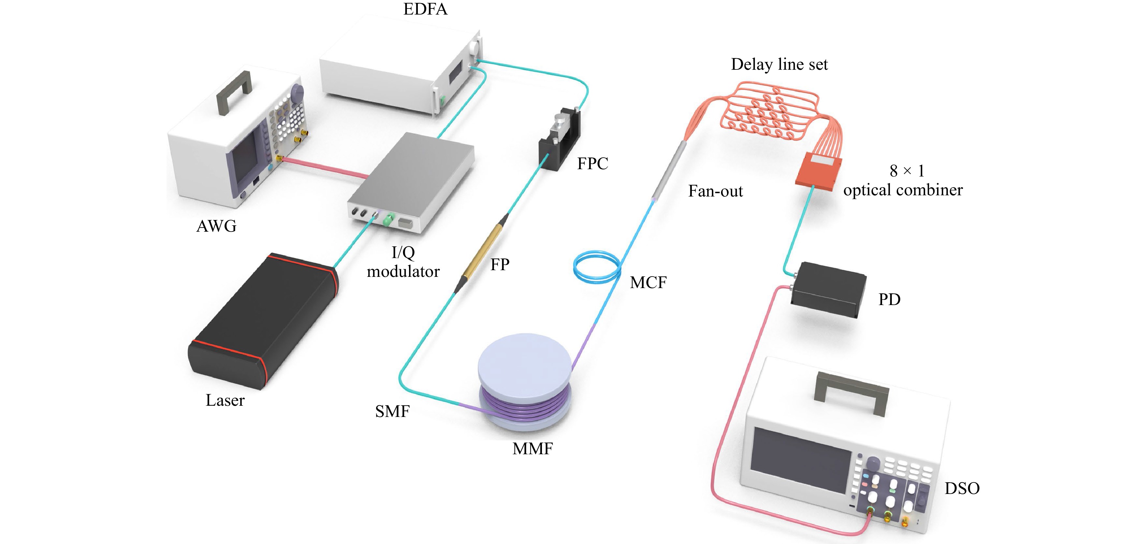
Fig. 2  Schematic of the experimental setup (AWG, arbitrary waveform generator; DSO, digital storage oscilloscope; EDFA, erbium-doped optical fiber amplifier; FPC, fiber polarization controller; FP, fiber polarizer; PD, photodiode; SMF, single-mode fiber).

Subsequently, a single-mode fiber (SMF) was used to connect the incident and measurement parts. The SMF is fused to a step-index MMF (10 m length, 105/125 µm core/cladding diameter, numerical aperture of 0.22). The other end of the MMF was fused to a seven-core MCF using a mild electrical arc discharge technique with center alignment owing to the slight difference in their cladding diameters. The MCF consists of 7 single-mode fiber cores with a cladding diameter of 150 µm and core pitch of 42 µm. The delay-line set contained a fan-out demultiplexer with seven short fibers of different lengths and an 8 × 1 optical combiner that temporally separated the seven pulses of the MCF into a pulse sequence. Light pulses were detected using a single photodetector with a bandwidth of 10 GHz and collected using a digital storage oscilloscope with a sampling rate of 20 GSa/s.

The critical parameters for data acquisition are listed in Table 1. The input pulses and corresponding pulse sequences are shown in Fig. 3a, b, respectively, where the pulse colours represent the different wavelengths. The pulse interval was set to 10 ns, and the pulse width was 0.5 ns. Therefore, the wavelength measurement rate was 100 MHz, determined by the input pulse's repetition period and could be further enhanced if needed. The SSB technique was used to sweep the frequency of each pulse signal. The wavelength difference between adjacent light pulses was approximately 0.8 pm (100 MHz in frequency). After passing through the MMF–MCF and delay line set, every pulse was converted into a sequence of seven pulses. To avoid overlapping pulses, the delay time should be shorter than the measurement time. The interval between delay lines was set to approximately 1 ns to ensure the total delay time was < 10 ns.

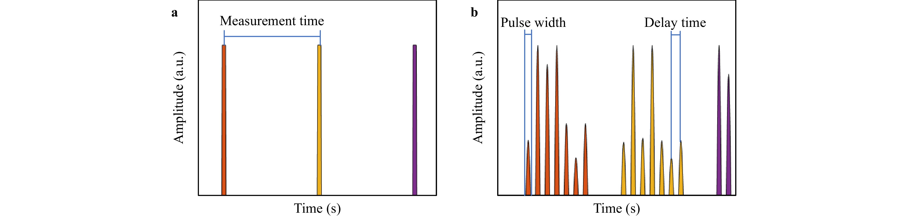
Fig. 3  Variation of light pulses. a Input light pulses and b detected pulse sequences.

The speckle pattern varied with the incident wavelength owing to the intermodal interference of the MMF. In the transverse plane of the MMF–MCF, each MCF core collected the speckle's pulse power at a fixed location. The delay lines converted the seven different pulses into a sequence that varied with the incident wavelength. Three pattern examples are presented in Fig. 4a–f at wavelengths of 1550.00 nm, 1550.25 nm, and 1550.50 nm. The left column shows the speckle patterns of the MMF at different wavelengths, and the right column shows the corresponding pulse sequences. More results can be found in the supplementary movie. The wavelengths can be identified based on a combination of their peak powers. We calculated the peak power of each pulse and normalized its intensity concerning the maximum power of each sequence. Subsequently, we input the seven-dimensional peak power of the pulse sequence and the corresponding wavelength labels into the MLP for training, thereby establishing a mapping to achieve wavelength estimation.

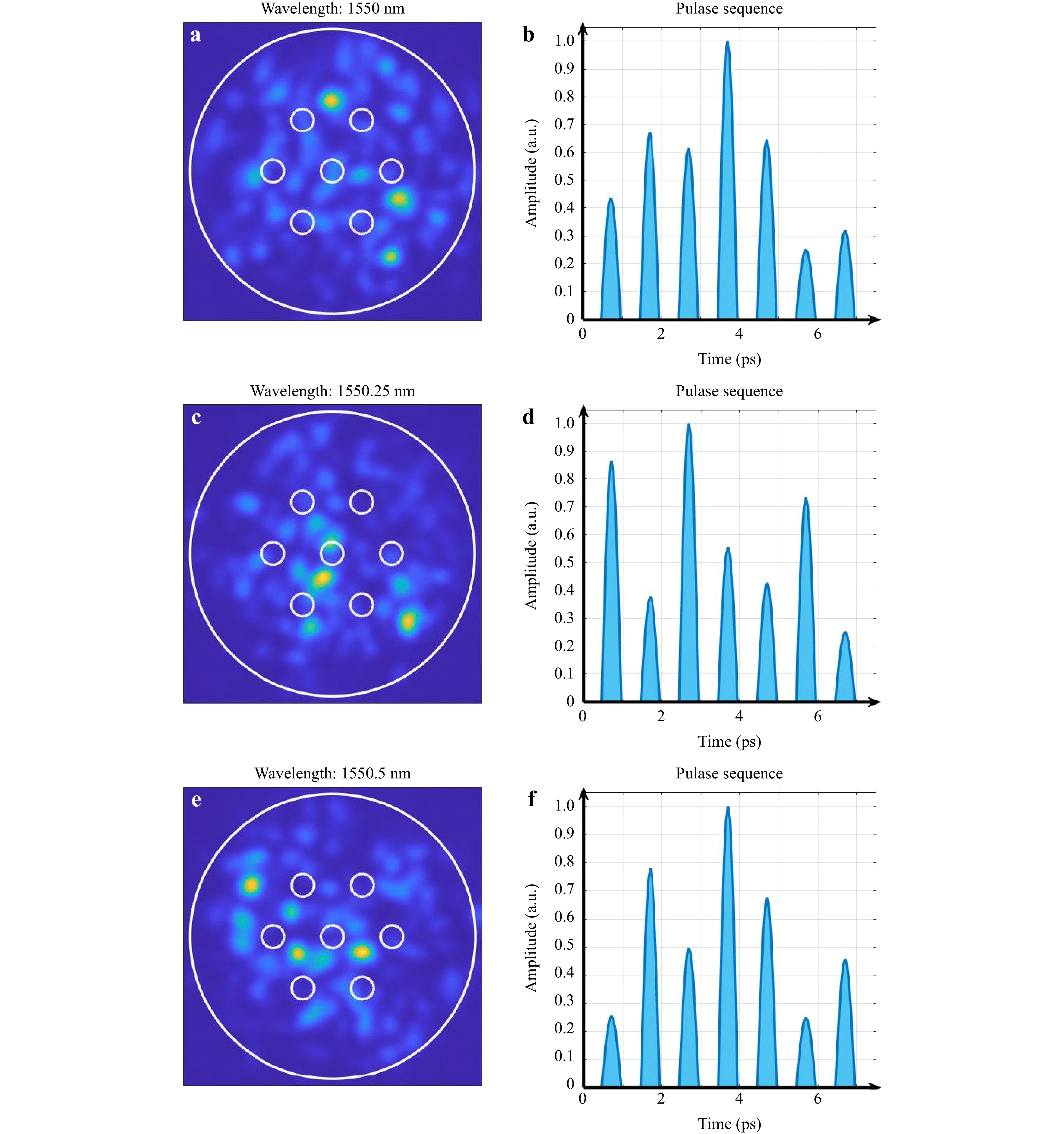
Fig. 4  Speckle patterns in MMF at different wavelengths (left column) and corresponding pulse sequences (right column). a, b 1550 nm, c, d 1550.25 nm, d, e 1550.5 nm. The white circles in each speckle pattern indicate the sampling positions of the MCF. (see supplementary movie)

Using high-speed sampling, we collected a large amount of data in a short time to easily establish a large dataset for adequate MLP training. In our experiment, 720 pulse sequences for each wavelength were captured at 1250 different wavelengths ranging from 1550 to 1551 nm (0.8 pm intervals). The sampling process was repeated 720 times at each wavelength to introduce the random noise caused by environmental perturbations. Therefore 900, 000 data sets were obtained.

MLP is a neuroscience-inspired machine learning method with supervised learning. MLPs are trained using input–output data to learn a nonlinear function approximator for classification or regression. We used a supervised deep neural network to map the relationship between pulse sequences and wavelengths. An MLP with multiple layers and neurons can capture abstract information, extract wavelength features, and is robust to environmental perturbations.

The structure of the proposed network is shown in Fig. 5. The MLP consists of eight layers, comprising a batch normalization layer and dense layers. The input was a sequence of seven pulses extracted from a seven-dimensional speckle pattern. The input first passes through the batch normalization layer to prevent overfitting and accelerate convergence. The dense layers then extract features from the pulse sequences. After feature extraction, the layers were fully connected to the output layer of one neuron using regression to estimate the wavelength. The connection between the two fully connected layers is given by

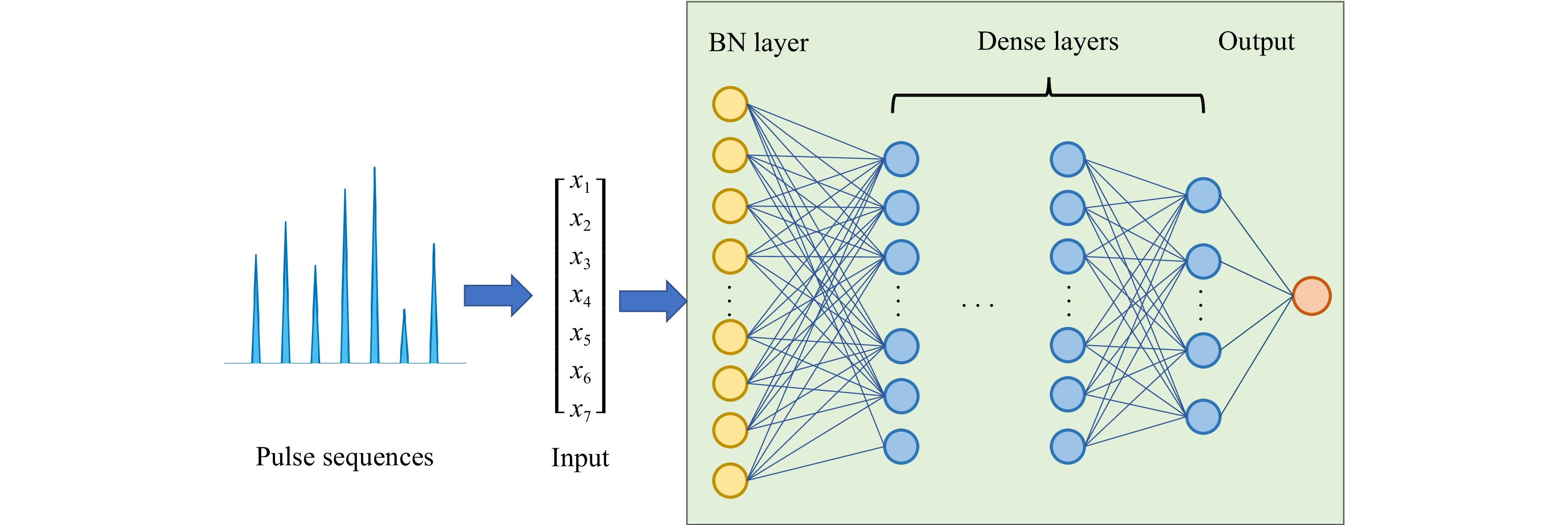
Fig. 5  Structure of proposed MLP (BN, batch normalization).

where ${w_{ij}}$ and ${b_{ij}}$ denote the weight and bias between the ${i_{th}}$ and ${j_{th}}$ layers, respectively. $outpu{t_i}$ and $outpu{t_j}$ represent the neuron vectors of the ${i_{th}}$ and ${j_{th}}$ layers, respectively. F is an activation function that is usually nonlinear.

As a regression task, the output of wavelength estimation is a continuous value. Thus, the corresponding activation function of the output layer is linear. Rectified linear units were used as the activation functions of the other layers to accelerate the calculation and prevent vanishing gradients. The adaptive gradient momentum optimization algorithm was used to train the model and minimize the output errors. The weights and biases of the layers can be adjusted automatically to make the prediction closer to the target during backpropagation. We considered the mean absolute error (MAE) instead of the common root-mean-square error because the MAE provides a higher performance for evaluating the average error of a model.

The proposed MLP was implemented on a Keras Python deep-learning library with a TensorFlow backend. Training and testing were performed using a computer with a graphics processing unit accelerator. After training, an MLP was established and used to estimate the incident wavelength from any pulse sequence.

Based on the system described above, 900,000 data samples were collected, randomly shuffled, and divided into three sets: 80% for training (720,000 samples), 10% for validation (90,000 samples), and 10% for testing (90,000 samples). Because of the random influence of environmental perturbations, each pulse sequence under the same wavelength label is different. This allowed us to assess the robustness of the model to environmental factors when estimating the wavelengths. Moreover, this classification method represented the entire data distribution well. We trained the MLP, established the relationship between the pulse sequence and wavelength using the training set, validated the overfitting using the validation set, and evaluated the performance of the well-trained MLP using the test set.

During training, we optimized the model hyperparameters to maximize performance. Therefore, the reported results were based on the best combination of hyperparameters. The training and validation MAE values over 1000 epochs are shown in Fig. 6. The model's performance on the training and validation sets was used to judge the overfitting or underfitting. After 200 epochs, the MAE of the training samples converged to 2.8 pm, whereas that of the validation samples converged to 2.7 pm. Hence, the MLP was well trained and showed good generalization, given the small gap between the results from the training and validation sets.

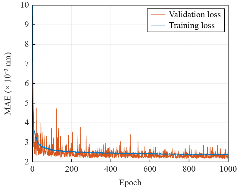
Fig. 6  Training and validation losses of MLP during training.

To evaluate the performance of the proposed wavemeter, the trained MLP was used to predict the wavelengths corresponding to the pulse sequences in the test set using samples that were not learned by the trained network. The experimental results for the wavelength estimation are shown in Fig. 7. The blue dots represent the estimation results, the black line is the fitted curve, and the red line represents the segmentation MAE corresponding to different wavelengths. The R-square of the data is 0.9998, demonstrating a strong linear relationship between the estimated and actual wavelengths. The equations for the fitting curve and R-square are as follows:

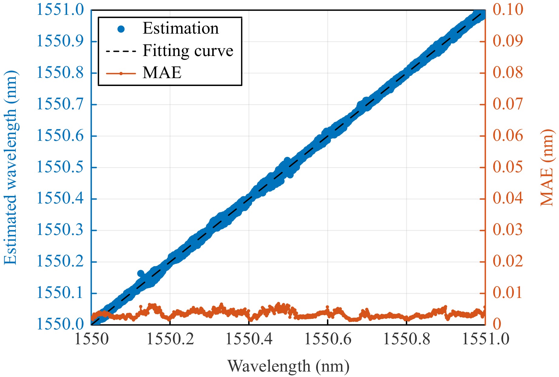
Fig. 7  Distribution of estimated wavelengths and corresponding segmentation MAE in the 1550–1551 nm range.

where Wavelength_Actual represents the actual wavelength, Wavelength_Estimated represents the predicted wavelength of the model, and Wavelength_Mean represents the mean of the actual wavelength. The MAE for the wavelength estimation was 2.7 pm, whereas the estimation range of the wavelength was 1550–1551 nm. Hence, highly accurate wavelength measurements were performed using a small amount of information and simple MLP. The reduction in required data allowed us to increase the measurement speed substantially. Expanding the estimation range is feasible because multimode fibers are sensitive to the entire C-band and other wavelengths. Changes in the wavelengths of other bands also lead to speckle variations. However, the wavemeter is currently designed for single-wavelength measurements. When the incident light comprises a spectrum of multiple wavelengths, it can potentially lead to a notable decline in measurement accuracy.

To demonstrate the high-speed measurements using our wavemeter approach, we varied the incident wavelength at a speed of 100 MHz. Incident optical pulses with a frequency of 100 MHz (measurement time = 10 ns) were sampled using the MCF, resulting in an output detection sequence with a pulse frequency of 1 GHz (pulse width = 1 ns). The experimental results are presented in Fig. 8. The black line represents the real wavelengths, and the red dots represent the estimated wavelengths. We used a tunable laser and SSB modulation to periodically change the incident wavelength from 1550 nm to 1550.8 nm at intervals of 0.08 nm. The MAE between the estimated and real values was still 2.7 pm, indicating that the measurement accuracy did not change with variations in speed. The experimental results demonstrate that the proposed wavemeter can obtain accurate measurements at high rates. Higher detection speed requires a PD with a larger bandwidth and a DSO with a higher sampling rate.

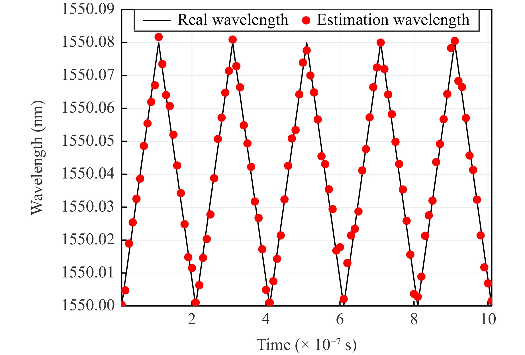
Fig. 8  Real (black line) and estimated (red dots) wavelengths varying over time.

Replacing a camera with an MCF substantially increases the measurement speed in a wavemeter but reduces the amount of acquired information. Approximately one million sampled pixels were reduced to seven data points, representing a drastic loss of information during sampling. We evaluated the performance provided by different numbers of sampling cores in the MCF to determine their effects on the accuracy. After training and testing using the MLP, we obtained the performance shown in Fig. 9.

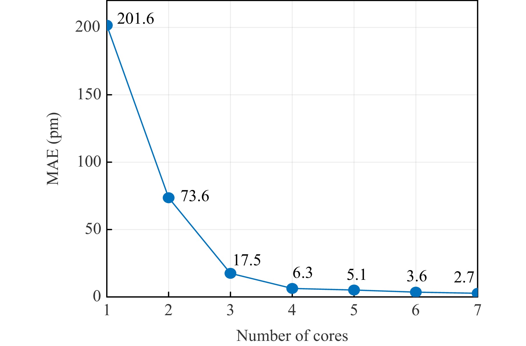
Fig. 9  Accuracy of wavemeter approach according to number of sampling cores in MCF.

As expected, the accuracy improved with the number of sampling cores, indicating that more cores can improve the measurement. For more than four cores, the accuracy slowly increased with further addition of cores. However, there was a tradeoff between measurement accuracy and speed because an increase in the number of sampling points simultaneously increased the length of the pulse sequence and reduced the measurement speed. Therefore, we use an MCF with seven cores to achieve high accuracy and speed.

In addition, the impact of wavelength variations on speckles may be more pronounced within a particular sampling area. Therefore, position sensitivity may occur because the seven cores of the MCF cannot cover the entire transverse plane of the MMF. To explore the correlation between wavelength prediction accuracy and core location, we examined the performance of the proposed method under various core locations by removing one core from the training set with the same architecture and hyperparameters as the MLP. Table 2 presents the results of the study.

After removing cores at different locations, the estimation results remained stable with small fluctuations. The results confirm that no particular core has a decisive influence on the estimation accuracy. This suggests that the sampling position does not need to be specifically fixed because the speckle variation is random.

We demonstrated a compact wavemeter with a high measurement rate and accuracy using an MMF and MCF setup. Based on the wavelength-dependent speckle patterns generated by the intermodal interference of the MMF, we used a seven-core MCF instead of a camera to sample the resulting speckle pattern, significantly improving the measurement speed and reducing costs. We experimentally demonstrated a measurement rate of 100 MHz with a resolution of 2.7 pm in a 1 nm operation bandwidth. Wavemeter performance can be further improved by increasing the spatial sampling channels of the MCF and optimizing the design of the MMF. The proposed measurement approach is promising for research and applications.

This study was supported by the National Key Research and Development Program of China (2021YFB2800902), National Natural Science Foundation of China (61931010, 62225110), and Hubei Province Key Research and Development Program (2020BAA006).