MT-Former: Multi-Task Hybrid Transformer and Deep Support Vector Data Description to Detect Novel anomalies during Semiconductor Manufacturing

Increasing demand for high-speed devices accelerates new semiconductor nanofabrication technologies to embed more memory into small devices¹. To ensure the quality of products from the nano-technology fabrications, using a scanning electron microscope (SEM) is required^2,3. Defect inspection is critical in semiconductor wafer fabrication process for product quality improvement at reduced production costs. In general, human inspection is time-consuming, labor-intensive and error-prone. Therefore, algorithmic methods for anomaly detection are increasingly essential^4–7.The rapid development of deep learning (DL) in computer vision^8–18 and the large amount of collected data in modern industry have made data-driven methods appealing to inspection engineers¹⁹.

Deep autoencoder (DAE) is one of data-driven approaches to detect anomalies²⁰. DAE creates the latent vectors from high-dimensional data, then reconstructs the data from the embedding vectors. When trained on only normal data, a DAE reconstructs normal cases well, meaning the reconstruction error $\| x-\hat{x}\| $ between the original image $ x $ and the reconstructed image $ \hat{x} $ is small for normal cases. On the other hand, the reconstruction error of the model is higher for abnormal cases^21–27. However, the DAE approach in semiconductor field has its limitation because of some defects that can be classified as normal owing to chip designing. Therefore, reconstruction loss function can be challenging for classifying semiconductor defects.

Generative adversarial networks (GANs)²⁸ are widely used for DL image analysis^29–32 and have also been adopted in the field of anomaly detection. AnoGAN³³ detects outliers by using a GAN that is trained on normal images. AnoGAN consists of two loss parts: residual loss and discrimination loss. In residual loss $ {L}_{R}\left({\textit z}\right) $, a generator G usually creates normal images $ G\left({\textit z}\right) $ from latent vector z, so an image error $\|\mathrm{x}-G\left({\rm z}\right)\| $ will be large if real data x is abnormal. The discrimination loss $ {L}_{D}\left({\textit z}\right) $ involves training a discriminator $ f $ on normal images, ensuring that the latent vectors $ f\left(x\right) $ of real normal images closely match the latent vectors $ f(G({\textit z})) $ of generated images. This similarity is enforced using the loss function $ \|f\left({\textit x}\right)-f\left(G\left({\rm z}\right)\right)\| $. Based on the two losses, the anomaly score, i.e. $ (1-{\lambda })\cdot {L}_{R} $+$ {\lambda }\cdot {L}_{D} $, is utilized to identify anomaly cases³⁴. GANomaly³⁵ makes AnoGAN's basic procedure more efficient by simultaneously generating images and encoding latent representation. GANomaly consists of a convolutional neural network $ E $ and a U-shaped generator $ G $ with an encoder $ {G}_{E} $ and a decoder $ {G}_{D} $. The model uses the encoder loss to compute the anomaly score $ \left|{G}_{E}\left(x\right)-E\left(G\left(x\right)\right)\right| $|.

Deep Support Vector Domain Description (Deep-SVDD)³⁶ is a one-class classifier designed to train a model for anomaly detection-based objectives. Deep-SVDD is devised to find abnormal cases that are beyond the range of normality. As faulty anomaly data accumulates, supervised learning-based research has also been conducted to classify defect types^37,38. Multiview data novelty detection using deep autoencoding support vector data descriptions (DMVSVDD) which jointly trains multiple DAEs to capture the correlated knowledge of multi-view data³⁹. And multi-task learning strategy has also been used with Deep-SVDD, which simultaneously learns one-class classification objective in addition to using DAEs to learn reconstruction⁴⁰. AdaDL-SVDD is trained on both normal and abnormal data to generate sparse representations with dictionary learning and adaptive boosting using some weak classifiers⁴¹, while Deep-SVDD using VAEs improves anomaly detection accuracy by ensuring distinctly separate latent representations in DAE⁴². The Patch-SVDD that use patches has advantages because it performs anomaly detection on a per-patch basis. Since they use small patches for evaluation, they localize anomalous regions well^43,44.

Semiconductor-fabrication field is using DL models to analyze defects in wafers. To determine a specified cause of problems in the manufacturing process, many researchers try to distinguish wafer map patterns and defect types in SEM images^38,45–48. Recently, SEM inspection needs anomaly-detection models that detect new defects that are different from the existing ones (Fig. 1). Many researchers developed anomaly models to distinguish defect types from normal cases^49–53, but it is difficult to identify new defects due to numerous defect types. To enable analysis of the issue arising from the new processes, the new types of anomalies must be detected. In addition, an anomaly-detection model should consider irregular shapes and different sizes of defects from a complex fab process⁵⁴. Therefore, a DL architecture is needed to extract appropriate features for this purpose.

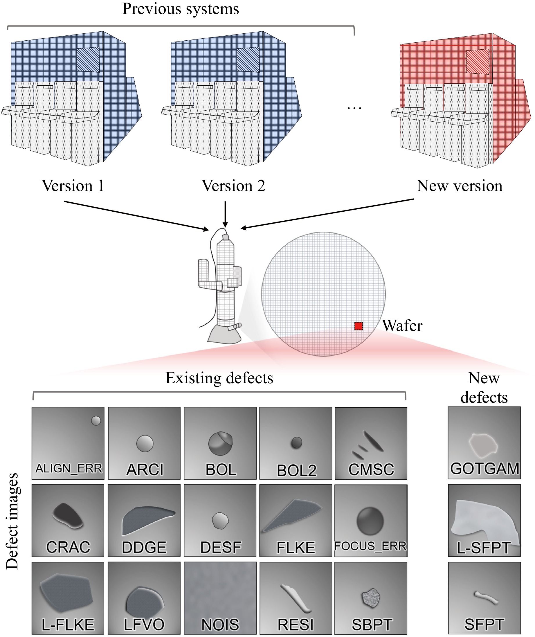
Fig. 1  Different defect types from various fabrication processes. New manufacturing technology can cause abnormal cases, which can be observed using scanning electron microscopy. In deep support vector domain description, existing defects are considered as normal cases and new types of defects as abnormal.

Herein, we propose an MT-former framework that exploits multi-tasking learning (MTL) and efficient self-attention to distinguish new semiconductor defects from the existing defect types. The main contributions are as follows:

● Unlike conventional anomaly models that just distinguish defects from normal cases, the MT-former proposes to distinguish new defects from the existing defects.

● MTL stabilizes SVDD training process by mitigating the fluctuation of false positive rate and false negative rate. In addition, MTL achieves efficient clustering of each normal class, and thereby overcomes the limitations of the basic Deep-SVDD model, which indiscriminately clusters the existing defect types with various patterns into a single class.

● Hybrid transformer considering long-range dependencies improve results by identifying irregular patterns on a wide range of defects, and efficiently exploiting focal loss to successfully process imbalanced data (Fig. 1).

● In classification of defect types, a shared encoder from MT-former is also superior to a CNN model that simply learns defect classification from scratch.

Deep-SVDD (Fig. 2a) is designed to map normal data into a hypersphere of minimum volume for one-class classification. A shared encoder learns transformation $ \varphi \left(\cdot ;W\right):X\to F $ for input data $ X\in {\mathbb{R}}^{h\times w\times k} $ and an output feature $ F\in {\mathbb{R}}^{1\times 1\times {k}'} $. The encoder includes $ L\in \mathbb{N} $ layers that have weights $ W=\{{W}^{1},{W}^{2}, ...,{W}^{L}\} $. We basically adopt the upstream and downstream stage of the basic Deep-SVDD, but the classification task is simultaneously trained at the two stages.

Fig. 2  Schematic overview of the MT-former framework. a The MT-former consists of an upstream and a downstream stage. At the upstream, U-shaped model with an encoder and a decoder is trained to reconstruct the existing defects. The encoder part simultaneously learns classification on the types of existing defect. At downstream, the encoder is fine-tuned by learning not only to categorize the existing defects cases, but also to cluster them. The encoder part is composed of the convolution and the efficient self-attention layer to extract both local and global features. b The efficient self-attention reduces the size of feature map on key and value.

During the upstream stage, DAE is used both to initialize weights of the shared encoder and to find a center point $ \mathrm{c}\in F $. DAE generates reconstruction images $ \hat{X} $ and searches for optimal $ {W}^{*} $ to minimize a reconstruction error. Given training dataset $ \mathrm{X}=\left\{{x}_{1}, \dots ,{x}_{N}\right\} $ and $ \mathrm{N}\in \mathbb{N} $, the error is defined as:

The center point is calculated as an average of all features’ coordinates as:

Downstream is a second training phase, where the normal samples are clustered to the center point. The goal of the SVDD is to form the smallest hypersphere with radius $ R $ that encompasses normal samples from center point $ c $.

Anomaly cases are identified if anomaly score $ s\left(x\right) $ exceeds $ R $, i.e. $ s\left(x\right) > {R}^{2} $:

Models that apply transformers use multi-head self-attention (MHSA) modules to capture long-range dependency at different scales⁵⁵. Such models require a huge training dataset, so a hybrid-transformer model, UT-Net, was introduced; it has an appropriate mix of convolutional layers and transformers⁵⁶. We utilize the UT-Net’s encoder which only applies convolution to the input image size. Unlike the encoder of UTNet, the self-attention module is applied on the input image size because our input image size is small.

UT-Net includes an efficient self-attention module (ESAM) to avoid inefficient and redundant computations. Given an input data $ X\in {\mathbb{R}}^{h\times w\times k} $, 1$ \times $1 convolutions project it to the vectors that consist of query, key, value: Q$ ,K,V\in {\mathbb{R}}^{h\times w\times d} $. Most of the informative features in self-attention are contained in the largest singular values⁵⁷, K and V are downscaled to $ \overline{K},\overline{V}\in {\mathbb{R}}^{{h}'\times {w}'\times d} $ by sub-sample operation (Fig. 2b). $ Q,\overline{K},\overline{V} $ is sequentially flattened and transposed to $ {Q}'\in {\mathbb{R}}^{o\times d} $ and $ \overline{K'},\overline{V'}\in {\mathbb{R}}^{u\times d} $ where $ o=h\times w,u={h}'\times {w}' $, and $ u\ll o $, which is followed by a scaled dot-product defined as:

In addition, relative positional encodings use independent relative height and relative width information as self-attention augmentations, which prevent perturbation equivariance while allowing for translation equivariance^58,59. The relative positional embeddings $ {r}_{{j}_{x}-{i}_{x}}^{W} $ and $ {r}_{{j}_{y}-{i}_{y}}^{H} $ between pixel $ i=\left({i}_{x},{i}_{y}\right) $ and pixel $ j=({j}_{x},{j}_{y}) $ are learned for relative width $ {j}_{x}-{i}_{x} $ and height $ {j}_{y}-{i}_{y} $. The relative attention logit for the strength of the relationship between pixel $ i $ and to pixel $ j $ is computed as:

where $ {q}_{i} $ is the i-th row of $ {Q}' $ and $ {k}_{j} $ is the j-th row of $ {K}' $. The final self-attention formula is defined as:

where $ {S}_{H}^{rel}\left[i,j\right]={q}_{i}^{T}{r}_{{j}_{y}-{i}_{y}}^{H} $ and $ {S}_{W}^{rel}\left[i,j\right]={q}_{i}^{T}{r}_{{j}_{x}-{i}_{x}}^{W} $ are matrices of relative position logits, with $ {S}_{H}^{rel},{S}_{W}^{rel}\in {\mathbb{R}}^{hw\times {h}'{w}'} $ (Fig. 2).

Our proposed method, MT-former (Fig. 2, Table 1), is composed of MTL and the hybrid transformer. MTL is a process of training a DL network on several related tasks at once with the intention that the shared knowledge learned from one task will increase accuracy on other tasks⁶⁰. The goal of our task is to distinguish new defects from existing defects, which are considered to be ‘normal’ cases in this one-class classification study. However, we assumed that due to the variety of defect types in shape, normal clustering would not be successful if all of the existing defects were grouped into a single class. This is because considering normal classes with various patterns results in a broad data distribution and the range of clustering. The broad distribution makes it easier for the new defect data to be included in the distribution of the existing defects. Therefore, we suppose that MTL, by classifying the existing defect types and clustering them, enables the model to properly cluster the various-normal cases.

In this study, we take two MTL stages, one upstream and one downstream. During the upstream stage $ {L}_{Up} $, reconstruction loss $ {L}_{DAE} $ and classification loss $ {L}_{Focal} $ are used. Focal loss $ {L}_{Focal} $ is applied to cover the existing defect classes imbalance problem⁶¹. $ {p}_{t} $ is the probability of classification by softmax when the model performs classification task on the existing defects. When focusing parameter γ increases, the learning weight of hard example with low probability also gets high. After initialization of the hybrid-transformed encoder, then during the downstream stage, the MT-former $ {L}_{Down} $ is proposed by simultaneously learning Deep-SVDD objective $ {L}_{SVDD} $ and the classification $ {L}_{Focal} $ on the hybrid-transformed encoder. The losses are defined as:

In a nutshell, the proposed method is trained on only the existing defect-labeled dataset. Based on the output value, the model detects the new defect.

We compared the accuracy of MT-former with six state-of-the-art deep anomaly detection models, i.e. DAE²⁰, GANomaly³⁵, AnoGAN³³, Patch-SVDD⁴³, Patchcore⁴⁴ and Deep-SVDD³⁶.

1. DAE²⁰ uses reconstruction error as a criterion for judging anomaly scores.

2. AnoGAN³³ is an early anomaly detection model based on GAN, which calculates anomaly scores by considering latent space in image space.

3. GANomaly³⁵ is a form in which an encoder is added to AnoGAN, and is more intuitive than AnoGAN to learn image and latent space at once.

4. Patch-SVDD⁴³ is an approach that can utilize local information by embedding in patch units. For comparison, Patch-SVDD's patch size is set to 32, which is half the input size.

5. Patchcore⁴⁴ extracts patch-wise features based on a model trained on ImageNet data to detect anomalies.

6. Deep-SVDD³⁶ obtains a hypersphere surrounding normal data, then uses it to identify abnormalities.

To evaluate anomaly-detection accuracy, we defined abnormal cases as ‘positive’ and used four evaluation metrics: true positive rate (TPR, recall), false positive rate (FPR), signal-to-background ratio (S/B), and area under the receiver operating characteristic curve (AUC). Receiver operating characteristic (ROC) curves are used to visualize the tradeoff between TPR and an FPR at different thresholds, while AUC shows the overall detection accuracy as the area under the ROC curve. In classification experiments, we adopted weighted average AUC because from the viewpoints of quality inspection and costs, frequent defects are the most important. The metrics are defined as:

where w_i is the number of data belonging to class i and s_i is the score of class i.

In this study, all experiments were conducted on 6078 datasets, including 24 new defect datasets from a domestic SK Hynix’s FAB process (SK-defect, SK Hynix, South Korea). SK data were collected in different settings and system environments. The defect images were provided in 64 to 80 pixel sizes, a size that allows engineers to visually identify defects and enables rapid analysis. The images typically have a field of view (FOV) ranging from 1 µm to 2 µm, which corresponds to approximately 15.6 nm to 31.3 nm per pixel for 64 × 64 pixel images. For each manufacturing process, defect types were defined considering image shape and process characteristics (Fig. 1). For instance, the ALIGN_ERR defect tends to exhibit alignment errors where the target is far from the center, the BOL defect often shows a round or circular shape, FLKE defect looks like flakes, which are similar to thin chip-like fragments⁶², and the FOCUS_ERR is characterized by blurry or out-of-focus patterns in the imaging. The collected data were divided into 2951 training and 3127 testing (Table 2a). The 18 defect classes include three new types of defects and 15 existing types of defects. This study considers the existing defects as ‘normal’ cases for the Deep-SVDD task. The data is not publicly available. However, the authors will make the data available upon reasonable request and with the permission of SK Hynix.

For robustly the capability of our method, we evaluated our models on two public dataset. The magnetic tile defect dataset was previously utilized for another validation⁶³. This dataset contains one non-defect case and five defect cases: blowhole, crack, fray, break, and uneven. To evaluate the ability to distinguish new defects, we performed validation by excluding the non-defect case and using only five defect classes, and set the ‘fray’ class that had the fewest instances as the ‘new’ defect. For normal defect data, we split the data 8:2 for training and testing, and all new defects were used for testing. In the final dataset, the number of training data was 287 and the number of testing data was 105, including 32 abnormal cases (Table 2b). The well-known HAM10000⁶⁴ consists of 6 subclasses, with an imbalanced dataset. The HAM10000 dataset is divided into 7007 training, 1003 validation, and 2005 testing (Table 2c). In our experiments with this dataset, we treated each subclass as a ‘new’ defect in turn, while considering the remaining subclasses as normal defects, which allowed us to observe the performance differences across classes.

The experiments were conducted using the PyTorch framework and executed on an NVIDIA Tesla T4 GPU with 16 GB of RAM. The initial learning rate was set to 0.001, and the Adam optimizer updated the model parameters with a weight decay of 0.0005. All images in datasets were resized to 64 × 64. Additionally, random horizontal-flip or vertical-flip data augmentations were applied. All models were trained for 100 epochs for upstream tasks and 800 epochs for downstream tasks, using a batch size of 128.

The same settings were also used for the external validation of magnetic tile defect and HAM10000 dataset. For the HAM10000 with small input size was scaled to 32 × 32 to account for the minimum input size of 32 for typical anomaly models for effective learning and sufficient feature representation Ref. 33. The proposed and comparison models were trained for 100 epochs with batch size 2. To deal with the small size of input data, all the comparative models parameterized to the same network architecture with our proposed model, including latent vector size 64 and model depth 3.

The anomaly performance of our proposed MT-former was compared with several state-of-the-art anomaly-detection models on the SK dataset (Table 3, Fig. 3). DAE achieved the lowest AUC (0.3220); this result indicates that DAE reconstruction scores do not work well on multi-normal classes because appropriate reconstruction is difficult when the normal shapes are diverse. The models that used GAN with discriminator show higher AUC (GANomaly 0.5897, AnoGAN 0.6912) than DAE. AnoGAN had higher TPR and AUC than GANomaly. Although GANomaly shows slightly lower FPR than AnoGAN, the lower TPR of GANomaly suggests that it mainly predicts the negative class. Patchcore demonstrates high TPR (0.7083) by leveraging a patch-level approach to analyze localized information. However, the FPR and AUC are poorer than our model, indicating challenges in handling multiple normal classes. A high FPR further reduces anomaly detection efficiency, especially in an imbalanced SK dataset, where the large number of normal cases leads to more misclassifications as abnormal. The base model, Deep-SVDD, exhibits a low TPR at the trained threshold, suggesting that the Deep-SVDD model is not well trained when various defect cases are considered as one class. Our proposed model, MT-former, shows the highest AUC (0.7821) by solving the problem of diverse defect types. Even if S/B metric of our proposed method is lower than GAN-based models, the proposed method achieved a higher AUC and TPR for overall small FPR than the other models (Fig. 3).

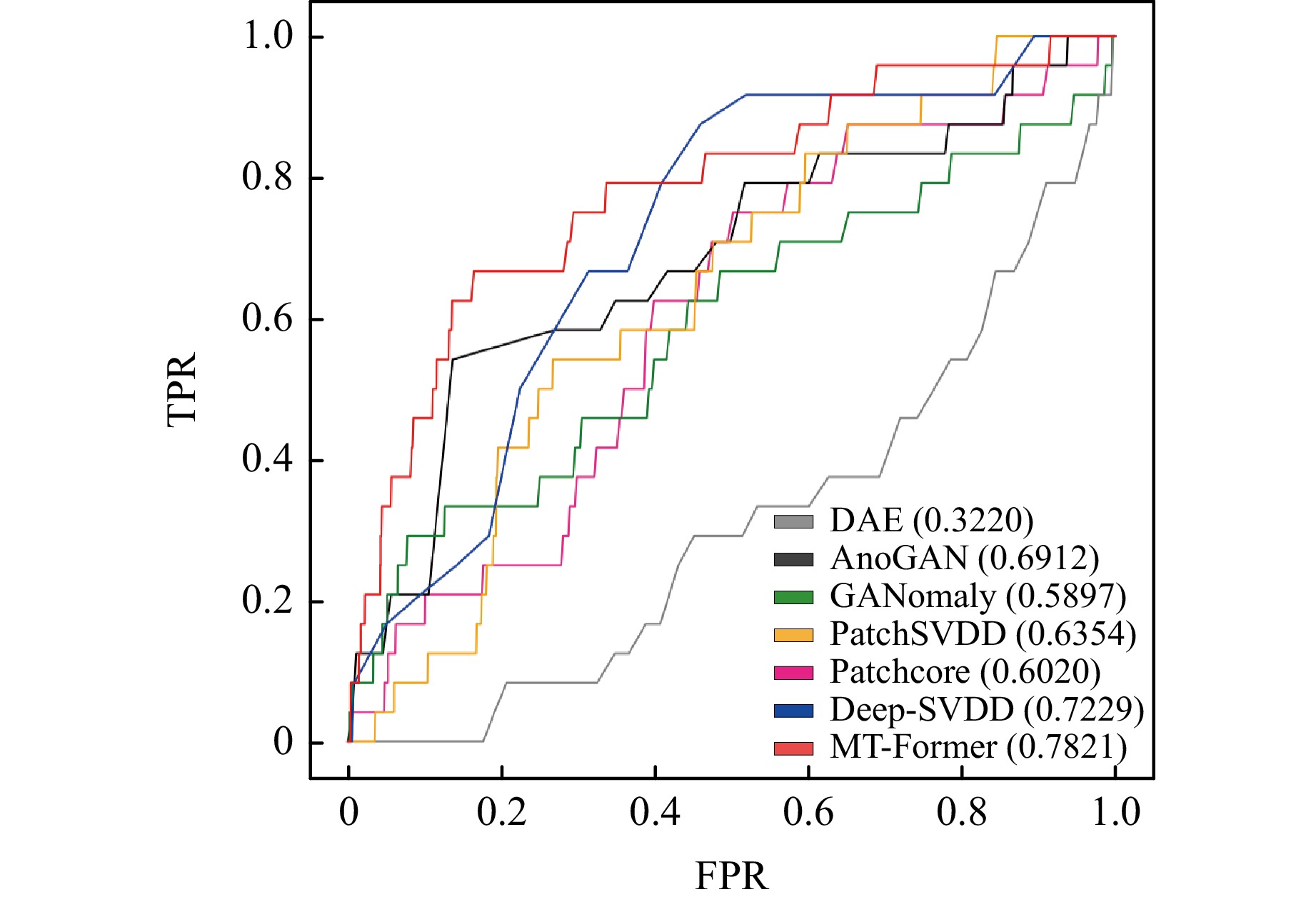
Fig. 3  Receiver operating characteristic (ROC) curve analysis of different state-of-the-arts and our proposed network on SK-defect dataset.

The Deep-SVDD based model (i.e., Deep-SVDD and MT-former) also has fewer parameters than models that use GAN (i.e., AnoGAN and Ganomaly) or based on patch-based models (i.e., Patch-SVDD and Patchcore). In terms of computational efficiency, MT-formers may be slightly slower than other models, but they offer high performance and compact model size with reasonably fast processing speed for automated defect detection. Since semiconductor manufacturing plants require significant resources, our lightweight MT-former model with high performance can be practically utilized for anomaly detection in this field.

In addition, the MT-former achieved the highest AUC (0.6798) on the magnetic tile defect dataset (Table 4 magnetic tile defect) and AUC (mean 0.7073) on the HAM10000 dataset (Table 4 HAM10000). Specifically, for the HAM10000 data, our model achieved the highest AUC scores in six of the seven classes except for class 5, demonstrating robust performance across different types of abnormal cases. These results show the model's generalization capabilities to a variety of external data sources.

In this section, we analyze the effectiveness of MTL, focal loss, and ESAM (Table 5). A basic Deep-SVDD model (Table 5a) had with TPR = 0 and FPR = 0; i.e., it identified all outcomes as ‘normal’.

MTL applied upstream showed increased AUC (0.7751) with a slightly better TPR (0.1667) than basic Deep-SVDD (Table 5b) but did not adequately cluster features (Fig. 4b). In addition, an unstable validation error (Fig. 5b) still seems to limit the anomaly-detection accuracy. Compared to applying MTL upstream, applying MTL downstream increased TRP by 29% (Table 5c), and clustered each normal class (Fig. 4c). When MTL was applied both upstream and downstream (Table 5d), its FPR (0.1795) AUC (0.7268) and clustering of normal classes all improved (Fig.4d) with the stabilized error (Fig. 5c).

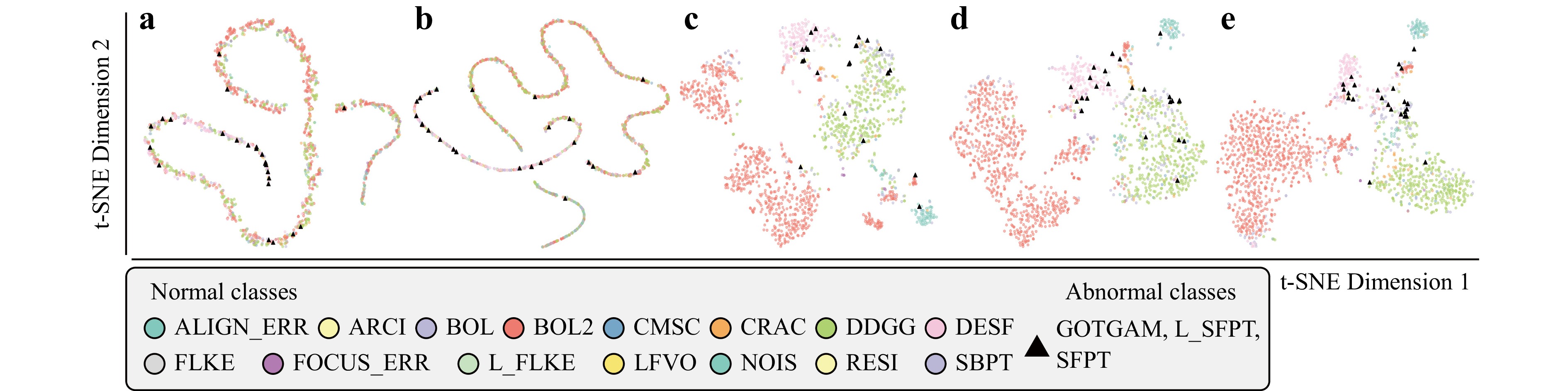
Fig. 4  Embedded feature visualization by t-SNE⁶⁵. a Deep-SVDD. b Deep-SVDD with multi-task learning applied only to the upstream phase (DAE). c Deep-SVDD with multi-task learning to the downstream phase (SVDD). d Deep-SVDD with multi-task learning at both the upstream and the downstream phase. e Proposed MT-former with multi-task learning, focal loss, and ESAM.

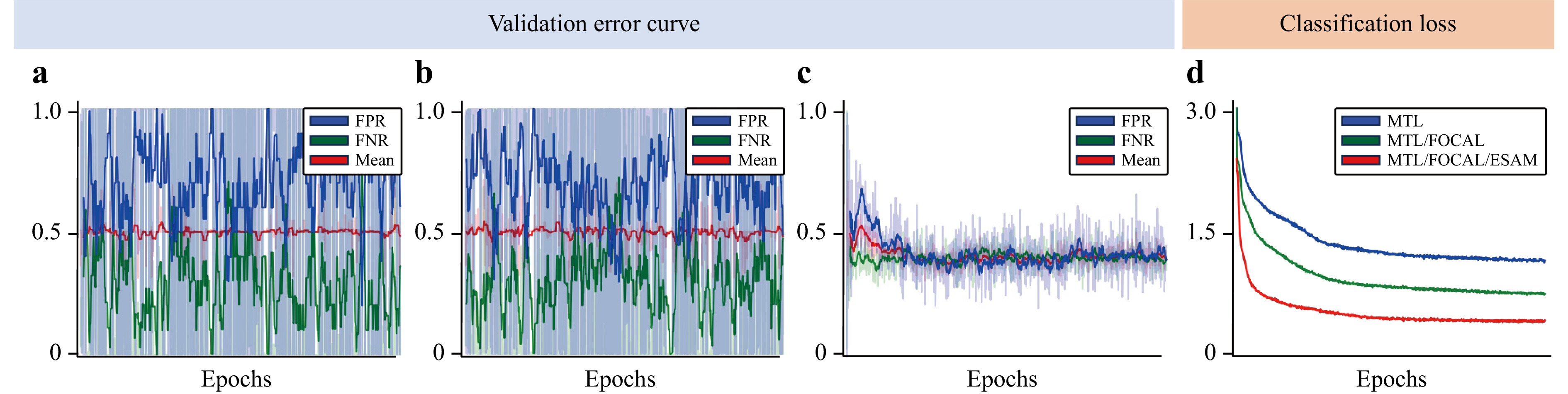
Fig. 5  Validation error curves for anomaly detection and classification task loss. a Deep-SVDD with ESAM. b Deep-SVDD with ESAM, including multi-task learning at the upstream phase. c Proposed MT-former with ESAM, including multi-task learning to both the upstream and the downstream phase. d Comparison of classification loss. a, b show fluctuation of FPR and FNR according to a training step.

These results demonstrate that the basic Deep-SVDD does not detect new anomalies when multiple classes are present, whereas MTL that considers different normal class types increases overall detection accuracy. The violin plot of Deep-SVDD (Fig. 6a) shows that distance between the latent vectors and the center point is very short (3.8 × 10⁻⁷) on y-axis compared to the other plots (Fig. 6b-d), and this distance does not even distinguish normal from abnormal at all. This result demonstrates that the Deep-SVDD only learns clustering to minimize the distance among all data without considering visual differences of data types. In this setting that includes a variety of normal classes, we found that separate clustering by types of normal classes in advance helps to increase detection of new types of anomalies.

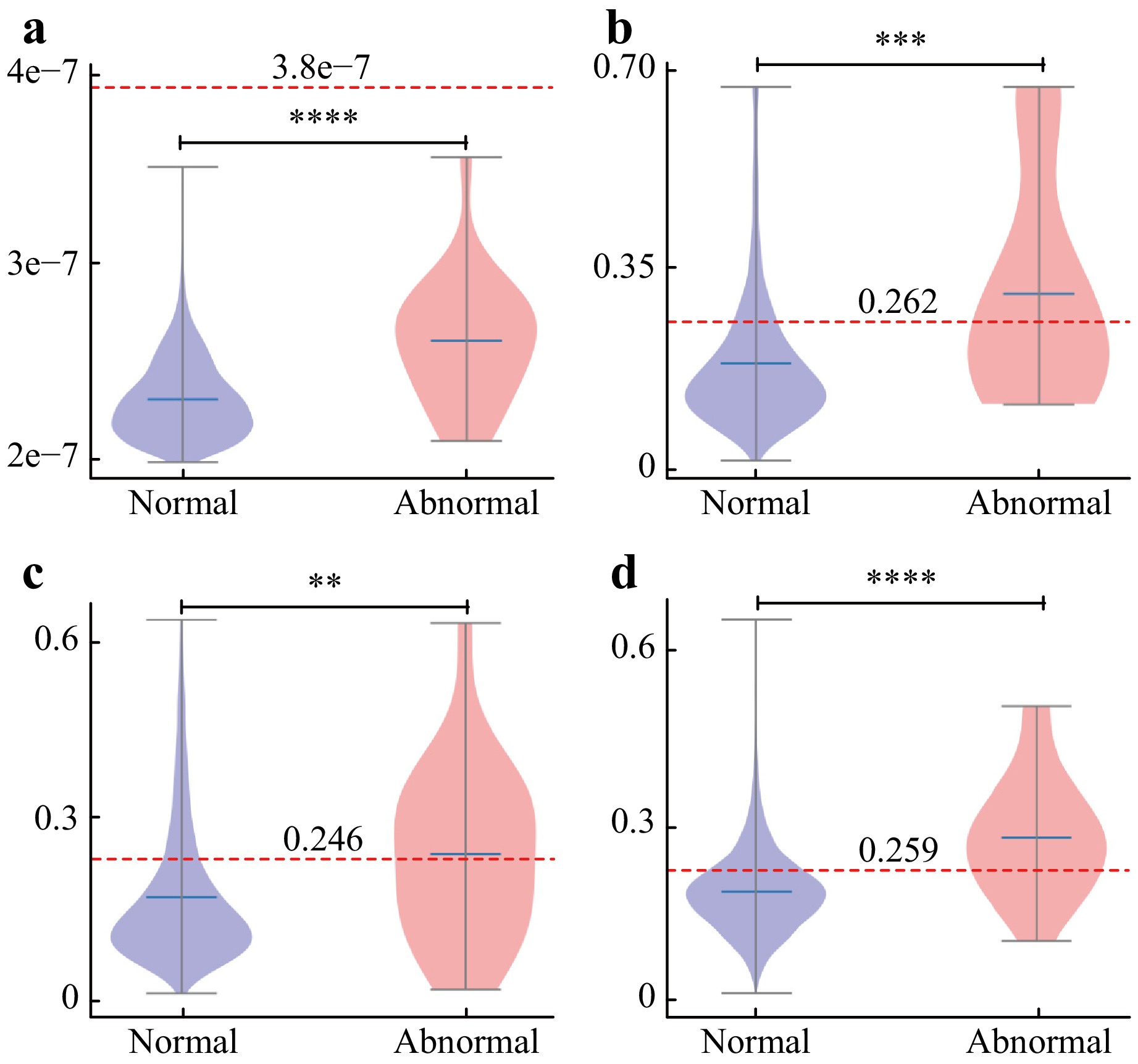
Fig. 6  Violin plots of distance distributions from a center point. The y-axis means distance between latent vectors of data and a center point. Red dotted line: threshold representing distance of decision boundary between abnormal (new types of defects) and normal (existing types of defects). a Deep-SVDD. b Deep-SVDD with multi-task learning applied both upstream and downstream. c Deep-SVDD with multi-task learning and focal loss. d Proposed MT-former with multi-task learning, focal loss, and ESAM. *, p < 0.05; **, p < 0.01; ***, p < 0.001; ****, p < 0.0001.

We also make use of focal loss to compensate for data imbalance (Table 5e), and ESAM to extract global context (Table 5f). Compared with Table 5d, use of only focal loss did not increase TPR (Table 5e). Use of only ESAM slightly improves the FPR, but still limits the TPR (Table 5f). On the other hand, the combination of focal loss with ESAM achieved the highest TPR (0.7083) and AUC (0.7821) (Table 5g). From the results, it is illustrated that the simultaneous use of focal loss and ESAM module mutually leverage each method’s effect by improving TPR. In other words, the ESAM module improves the efficiency of the focal loss. This effect can also be observed in (Fig. 4e), which shows that both normal and abnormal cases are better clustered than when MTL was used alone (Fig. 4d). Furthermore, embedded features show a significant difference between normal case and abnormal case (p < 0.0001) (Fig. 6d).

In addition, we conducted an ablation study that considered different numbers of heads for ESAM (Table 6). The best results (TPR = 0.7083, AUC = 0.7821) were obtained with three heads; i.e., both too many heads and too few heads impair ESAM results.

The effectiveness of MTL, focal loss, and ESAM on normal class classification accuracy was examined (Table 7). Overall accuracy was quantified using a weighted average of the AUCs of each class. As a baseline, a basic Deep-SVDD encoder was trained from scratch for classification purposes only (Table 7a). Fine tuning of an encoder extracted from MTL at both upstream and downstream (Table 7b) achieved the best score for the BOL class (0.8776), but poor results for most classes. The application of focal loss for imbalance multi-class data (Table 7c) achieved the highest score on L_FLKE (0.9487) and second best on five classes (ALIGN_ERR, ARCI, BOL2, FLKE, and NOIS), improved weighted average (0.8985) and showed better loss reduction (Fig. 5d).

Fine-tuning the encoder from MT-former achieved superior accuracy in most classes, and yielded the highest overall weighted average (0.9290) (Table 7d) and the best loss convergence (Fig. 5d). These results indicate that ESAM achieves the best identification of new defect types, and it improved its ability to classify irregular patterns by considering the global context. Furthermore, from the embedded features in the previous analysis (Fig. 4e), we deduce that effectively clustering each class with the MT-former can also be helpful in classification tasks.

Conventional anomaly detection only distinguishes between non-defective and defective images, the models are just required to identify regular patterns of normal images. Deep autoencoders (DAEs), a classic anomaly detection model, perform poorly when applied to multi-normal classes, because it is difficult to accurately reconstruct different normal shapes. Deep Support Vector Domain Description (Deep-SVDD) is known to classify anomaly cases given single-normal case. Since the normal cases have similar shapes and patterns in conventional task, the latent vectors are clustered properly even if they are trained as one class. However, it is observed that the vectors are not properly clustered if the existing abnormal cases are heterogeneous in shape and pattern, as in our task. We analyzed that training diverse patterns of existing defects as a single class led to a broad data distribution on the existing defects, causing new defects to be included into the broad distribution. To solve this problem, we used multi-task learning (MTL) to simultaneously learn to distinguish the existing abnormal classes, avoiding the broad distribution and leading to the well-clustered latent vectors. In addition, since our model is only trained on the existing defects, the model does not require retraining when a new defect is identified. Considering intricate patterns of the current defect classes, we introduced MT-former that uses MTL and an ESAM to detect unknown defects that existing inspection systems cannot find in scanning electron microscope (SEM) images. MTL can simultaneously classify the existing defect kinds with various forms, so it can cluster existing classes efficiently for anomaly identification. MTL also greatly stabilizes training with respect to false positive rate (FPR) and false negative rate (FNR). ESAM takes global contextual features to consider irregular patterns from complex fabrication systems, and maximizes the efficiency of focal loss to effectively analyze imbalanced data.

Compared with SOTA models, our method shows better TPR result for especially the region < 20% FPR region with high AUC (Fig. 3), representing that our model provides more balanced performance at various thresholds. Table 3 demonstrates that while GANomaly records low FPR at an optimal threshold, the TPR remains below 50% (Table 3). This indicates that missing even a few defects could lead to significant economic losses in the semiconductor industry, making the model unsuitable for practical applications. Hence, our model proves to be more effective than other methods for this field. These improvements are attributed to the integration of the ESAM and convolutional module as a block, enabling effective extraction of both local and global features. As a result, our model successfully detects defects across both localized areas and broader regions, enhancing overall reliability. Finally, the pretrained model for anomaly detection demonstrates that the model can also serve as a weight-initialization technique to classify the existing-defect classes.

For future works, we discuss potential challenges. First of all, a small increase in FPR indicates a large number of normal cases are misclassified as abnormal because of the imbalanced data. Therefore, further improvements in reducing FPR are essential to achieve reliable anomaly detection. Second, the sub-sampling approach of the ESAM should be further studied. In its current implementation, the sub-sampling reduces resolution at a fixed ratio across all layers. However, applying the same subsampling rate to smaller feature maps of last layers can cause substantial loss of abstract information. Therefore, it is needed to study finding the optimal sub-sampling approach with less information loss. Last, the model's explainability should be covered more. While visualization techniques like t-SNE provide valuable insights into the model's behavior, incorporating methods such as Class Activation Mapping (CAM) could highlight the regions the model focuses on during classification or anomaly detection tasks. This advancement would improve interpretability and offer deeper insights into the model’s decision-making process, fostering greater transparency and trust in its application.

This work was supported by SK Hynix AICC (P23.03); by the National Research Foundation of Korea (NRF) grant funded by the Ministry of Science and ICT (2023R1A2C3004880) and the Ministry of Education (2020R1A6A1A03047902 and 2022R1A6A1A03052954); by Basic Science Research Program through the NRF funded by the Ministry of Education (RS-2024-00415450); by Institute of Information & communications Technology Planning & Evaluation (IITP) grant funded by the Korea government (MSIT) (No.RS-2019-II191906, Artificial Intelligence Graduate School Program (POSTECH)); by the BK21 FOUR project; by Glocal University 30 projects.