Online platform for generating realistic digital phantoms of OCT signals and performing multimodal processing towards optical cancer diagnostics

Optical coherence tomography (OCT) features mesoscopic resolution, meaning that the resolution volume encompasses only a few cells in biological tissue (e.g., tumour cells). Specifically, the typical axial resolution ranges 5–10 micrometres, whereas the lateral resolution, determined by the optical beam profile, is 5–20 micrometres¹. This level of resolution exceeds the typical resolution of medical ultrasound and approaches that of microscopy. In comparison with microscopy, OCT provides a greater penetration depth (typically ~1–2 millimetres), and therefore, fills the niche between medical ultrasound and microscopy1². OCT enables non-invasive optical biopsies³ to evaluate tissue structures, inclusions, and clusters of cells⁴. Moreover, OCT signal features exhibit high sensitivity to the properties of sub-resolution optical scatterers. For instance, speckle pattern parameters correlate with scatterer concentration⁵ and scatterer clustering⁶, whereas temporal speckle variance is sensitive to scatterer motion, such as blood flow⁷. Many studies have utilised these principles empirically, e.g. to visualise blood vessels using temporal variability of speckle pattern parameters⁸, or to use spatial variations in speckle patterns to isolate layers in biological tissues^9,10, tumour areas^11,12 or other tissue structures^13,14. However, relevant signal features can also be evaluated and used to improve signal processing approaches based on specific tests on digital phantoms.

Doronin and Meglinski¹⁵ introduced an online object-oriented Monte Carlo computational tool designed for biomedical optical applications. This tool enables the simulation of light-tissue interactions and provides insights into the localisation and scattering of optical radiation within biological tissues. Such tools are essential for understanding the complex processes underlying OCT signal formation and optimising imaging techniques. Several other MC-based open-source platforms have been developed to facilitate OCT simulations and signal processing. For example, Monte Carlo-based codes^16,17 (the principles of which are discussed in Refs. 18,19 and Refs. 20−22) utilise massively parallel simulations to model OCT signals, emphasising the influence of multiple scattering effects. Another notable simulation framework²³ adopts a wave-based description²⁴ of OCT image formation and provides a computational environment for simulating OCT signals under various conditions, including polarisation effects and signal decay due to scattering. Collectively, these tools enhance the ability to generate realistic digital phantoms and evaluate OCT signal features under controlled conditions. However, a drawback of the abovementioned simulation codes is that they are not integrated into no-code platforms, are computationally demanding, and mostly require execution using a GPU, which may limit their accessibility and ease of use for non-expert users.

In addition to simulation tools intended for simulating OCT signals, several platforms have focused on OCT signal processing and analysis. For instance, the Altris AI platform²⁵ provides advanced tools for ophthalmology applications, leveraging artificial intelligence to analyse OCT data for clinical purposes. The Relayer platform²⁶ offers a cloud-based platform for OCT data processing, enabling efficient and scalable analysis of workflows. The MATLAB-based OCTSeg tool²⁷ was designed for the segmentation and evaluation of retinal OCT images, facilitating the extraction of meaningful features from OCT datasets. Furthermore, the RAG-Net v2 package²⁸ described in Ref. 29 provides a deep-learning-based framework for OCT image analysis, demonstrating the growing role of machine learning in OCT research. However, OCT segmentation tools designed for non-ophthalmology and non-coronary vascular emerging applications are lacking, and no platforms or integrated solutions are currently available for non-ophthalmic or non-coronary vascular OCT.

In this paper, we present an Internet-based no-code framework for producing OCT digital phantoms and multimodal OCT signal processing, mostly oriented towards cancer-related evaluation of OCT images.

The simulation framework considers the scatterer parameters and properties of the OCT device as inputs and provides complex-valued OCT scans as outputs. The input scatterer and device parameters can be used as the ground truth for the controlled evaluation of speckle patterns. Here, we discuss four variants which imply different degrees of realism of signal formation procedures: basic speckle pattern generation in the signal-scattering approximation; naive attenuation-pattern implementation based on the assumption of strong dominance of scattering contribution over absorption, which is typical for OCT; attenuation implementation based on scattering losses at individual scatterers, and OCT signal formation for arbitrary illuminating beam profiles. These numerical phantoms can be utilised for solving various tasks using several OCT signal processing methods implemented on the described platform.

As instructive examples of the implemented OCT signal processing procedures, we discuss interframe strain estimation, optical attenuation coefficient estimation (OAC), speckle statistics evaluation, including speckle contrast estimation, and depolarisation ratio evaluation (for co- and cross-polarisation channels where available), as well as aberration corrections. Based on these basic procedures, we demonstrate a multimodal OCT signal analysis of real OCT scans specifically aimed at the evaluation of cancer tissues. These examples comprise experimental records of brain, skin, and endometrial tissue samples.

In the rapidly evolving field of medical diagnostics, the ability to process and efficiently analyse data using various imaging techniques is crucial for medical professionals who may not possess special qualifications in signal analysis. A no-code medical image-processing platform empowers clinicians by eliminating the need for advanced programming skills, enabling them to focus on their primary responsibilities—patient care and diagnosis. By providing an accessible interface for sophisticated imaging techniques, such platforms allow clinicians to harness the power of cutting-edge technologies such as OCT without technical complexity. The expansion of no-code platforms has democratised access to advanced diagnostic tools for healthcare professionals without extensive technical training^30,31. Thus, no-code platforms are pivotal in bridging the gap between sophisticated medical imaging technologies and everyday clinical practice, ultimately contributing to improved patient outcomes.

The architecture of our no-code OCT software platform https://www.opticelastograph.com was designed to efficiently manage and process OCT data using a modular and scalable approach. As illustrated in Fig. 1, the platform is organised into several key components that work together to provide robust OCT signal processing capabilities.

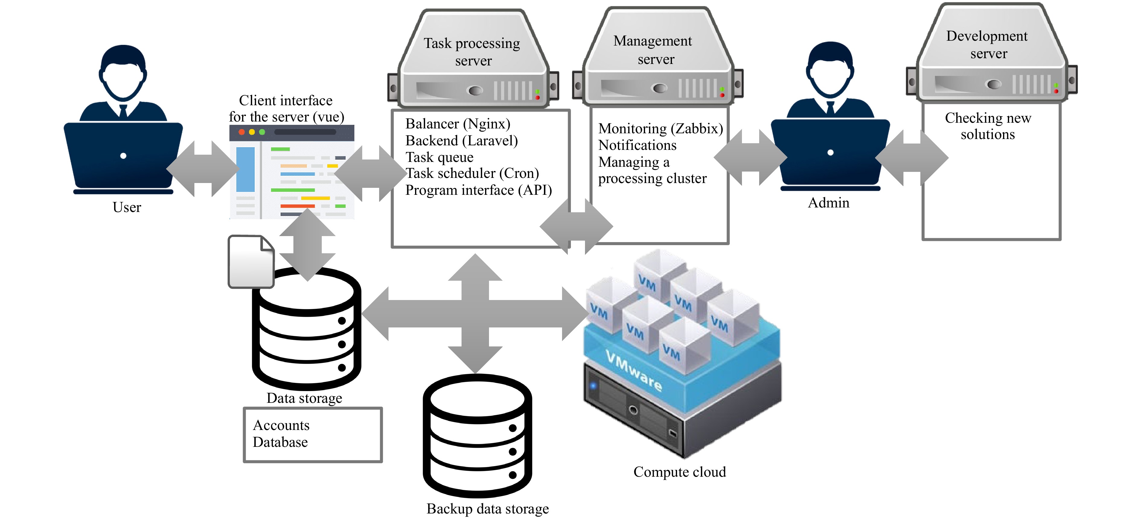
Fig. 1  Architecture Diagram of the No-Code OCT Software Platform. This diagram illustrates the architecture of our no-code OCT software platform, emphasising its modular components and workflow. Central to this architecture are Docker containers that encapsulate Octave code for OCT signal processing, ensuring consistency and scalability. The platform is equipped with an administration layer for system management, a user interface for data upload and interaction, an S3-compatible storage system for secure data handling, and a task processing cluster that dynamically adjusts its capacity based on workload. The system is supported by a robust backend, load balancing, task scheduling, and monitoring infrastructure, all designed to optimise the processing of OCT data for various applications, including cancer tissue evaluation.

At the core of the system, Docker containers encapsulate OCT processing code written in Octave to ensure consistency and ease of deployment across different environments. These containers are stored in a Docker registry, based on the Yandex Container Registry, allowing for version control and seamless updates.

The platform comprises multiple layers, starting with an administration layer, where system administrators manage settings, add processing handlers, and oversee user access and load balancing across processing clusters. Administrators also maintain user lists and task-processing balances to ensure efficient load distribution.

Users interact with the platform through a dedicated user interface that allows them to upload OCT datasets to an S3-compatible storage system. This storage, built on Yandex Object Storage, provides each user with a personalised bucket for secure data storage and retrieval.

The task processing server, built on the Ubuntu 22.04.01 LTS Linux distribution, manages incoming processing requests. It facilitates load balancing, monitors user balances, and queues tasks. This server was integrated with the backend system, developed using the Laravel PHP framework, and employed Nginx for load balancing and access control.

Tasks are scheduled and automated using a task scheduler (cron) that operates in conjunction with a task queue. This queue provides an API for task management and monitoring, thereby ensuring smooth task execution.

A database server running PostgreSQL 15 on Ubuntu 22.04.01 LTS Linux handles all project data, whereas a management server monitors the queue and overall system health, sending notifications to alert administrators of any issues.

The backup server ensures data integrity by maintaining backups of the entire platform, using a virtual machine with redundant disk storage.

Finally, the task-processing cluster consists of a dynamic set of virtual machines with varying performance configurations. Presently, the platform uses four cores of an Intel Xeon Gold 6338 CPU, with scalable RAM from 4 to 32 GB (depending on the size of the uploaded scan set) and a virtual 40 GB SSD. The capacity of this cluster adapts to the number of tasks and parameters set by administrators to optimise resource usage and processing efficiency. Using Docker containers, the platform ensures that all OCT processing tasks are executed in isolated and reproducible environments, thereby enhancing both security and reliability.

Fig. 2 shows a screenshot of the user interface with examples of uploaded real OCT scans acquired in two orthogonal polarisations: the structural OCT scan representing the total signal intensity in the upper row and the derived images representing the spatially resolved attenuation, speckle contrast parameter, and depolarisation ratio in the lower row. Multimodal processing of the scans, as shown in Fig. 2, required approximately 10 s.

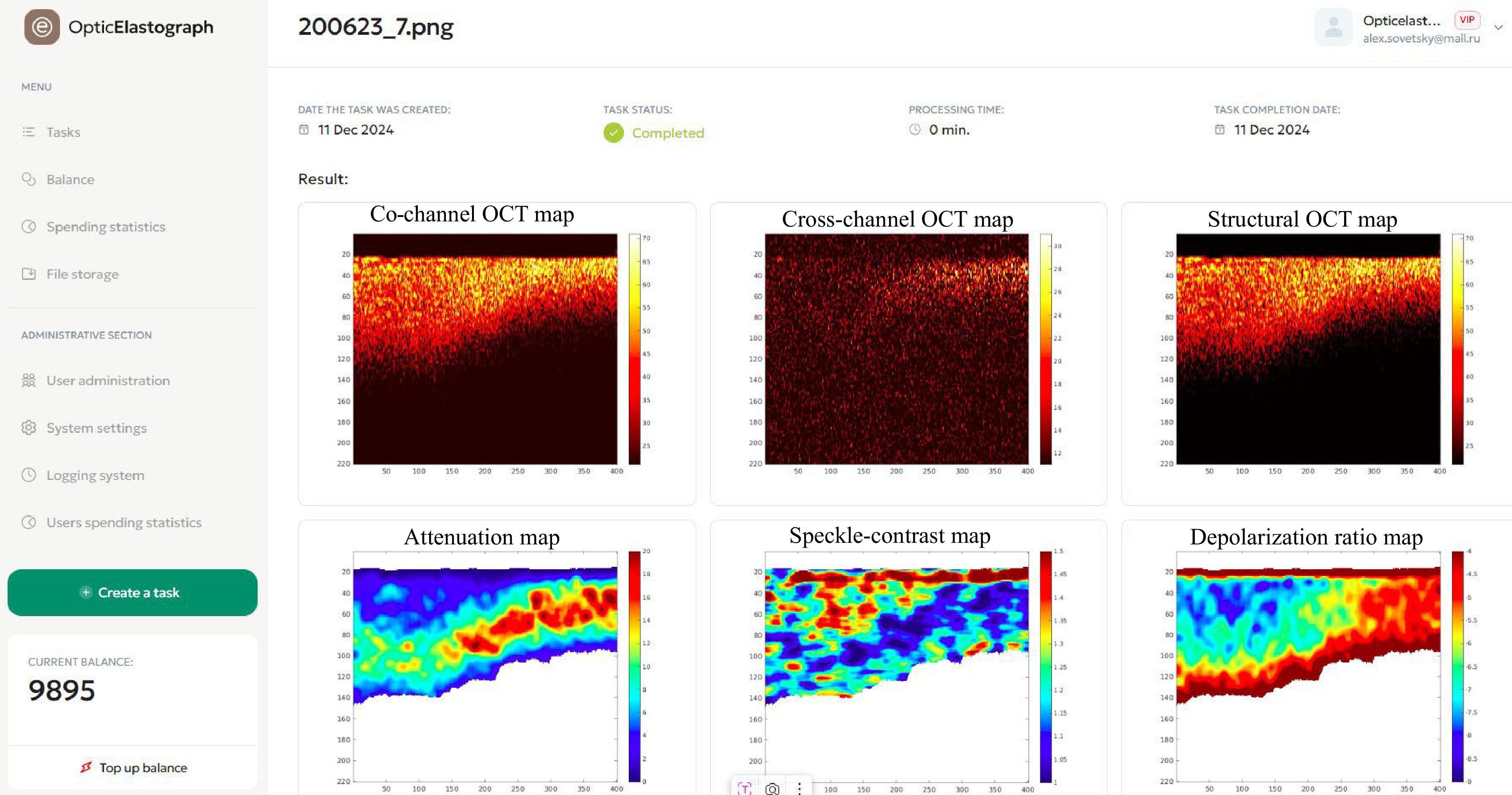
Fig. 2  A screenshot demonstrating the user menu (left vertical column) and system interface. In the right-hand part, the upper row shows examples of uploaded real OCT-scans acquired in two orthogonal polarisations, the structural OCT scan representing the total signal intensity. The lower row shows the derived images representing the spatially-resolved attenuation, speckle contrast parameter and the depolarisation ratio.

The full complex-valued signal of the spectral-domain OCT was simulated via the summation of the received amplitudes $ A_j^{rcv} $ of the scattered waves at each wavelength of the OCT system for all scatterers within the OCT beam. This general idea is described in the literature^32,33. The complex-valued amplitude A_px(q) of the qth pixel in the axial direction of a one-dimensional A-scan can be calculated as the inverse Fourier transform of the received spectral components backscattered from localised point-like scatterers distributed in the simulated tissue:

where $ {{\textit z}_q} $ is the depth coordinate corresponding to the centre of the q-th pixel, n is the index of the discrete spectral components (n varies from $ - N/2 $ to $ N/2 $, wherein we assume that $ N $ is an even value and $ N + 1 $ is the total number of discrete spectral components registered by the receiving array or swept-source system detector), $ {k_n} = {k_0} + {\text π} n/H $ is the wavenumber of the n-th optical-signal component, $ {k_0} $ is the wave number corresponding to the centre wavelength of the broadband light source with the amplitude spectral form $ S({k_n}) $, $ {{\textit z}_j} $ is the axial coordinate of the j-th scatterer, $ A_j^{rcv} $ takes into account the beam profile of the OCT system via the additional dependence of $ A_j^{rcv} $ on the lateral coordinates of scatterers, and $ H = {\text π} /\delta k $ is the maximum imaged depth corresponding to the step $ \delta k = |{k_{n + 1}} - {k_n}| $ between the spectral components. Eq. 1 is written under the single-scattering approximation, which forms the basis of OCT image generation, whereas multiple scattering contributes to OCT signal degradation and, in most cases, may be neglected.

By introducing the dependence of $ A_j^{rcv} $ on the lateral positions of the scatterers, Eq. 1 allows the depth-independent lateral beam profile to be accounted for relatively easily. In the simplest case, the amplitude lateral profile of the beam may be assumed to be rectangular or Gaussian to imitate a weakly focused Gaussian beam, for which the lateral curvature of the phase front may be reasonably neglected (as in Ref. 33). Presently, the online platform utilises the latter variant of the OCT beam with a Gaussian amplitude profile of the form $ \exp [({x^2} + {y^2})/W_0^2] $, where x and y are the lateral coordinates and $ W_0^{} $ is the beam radius. This approximation corresponds to the most widely used OCT systems with weakly focused beams, allowing for a nearly invariant transverse resolution within the imaged depth. A rigorous treatment of Gaussian beam focusing was presented in Ref. 34. A comparison with the cited model³⁴ indicated good agreement with the used approximation³³, in which only the amplitude lateral OCT beam profile was retained. The approximate model³³ and its initial simpler version³² (see the discussion therein) already yield statistical properties of speckles similar to those in the OCT scans of real tissues. The model³³ also readily accounts for the inter-frame motions of scatterers, which is of key importance for testing methods of angiographic and elastographic processing³⁵.

Another important aspect is that the speckle patterns simulated using Eq. 1 do not imitate the influence of the attenuation typical of real OCT B-scans. An example of a B-scan representing the basic speckle pattern, neglecting the attenuation influence, is shown in panel (a-2) of Fig. 3. The methods for introducing the influence of attenuation are discussed in the following sections.

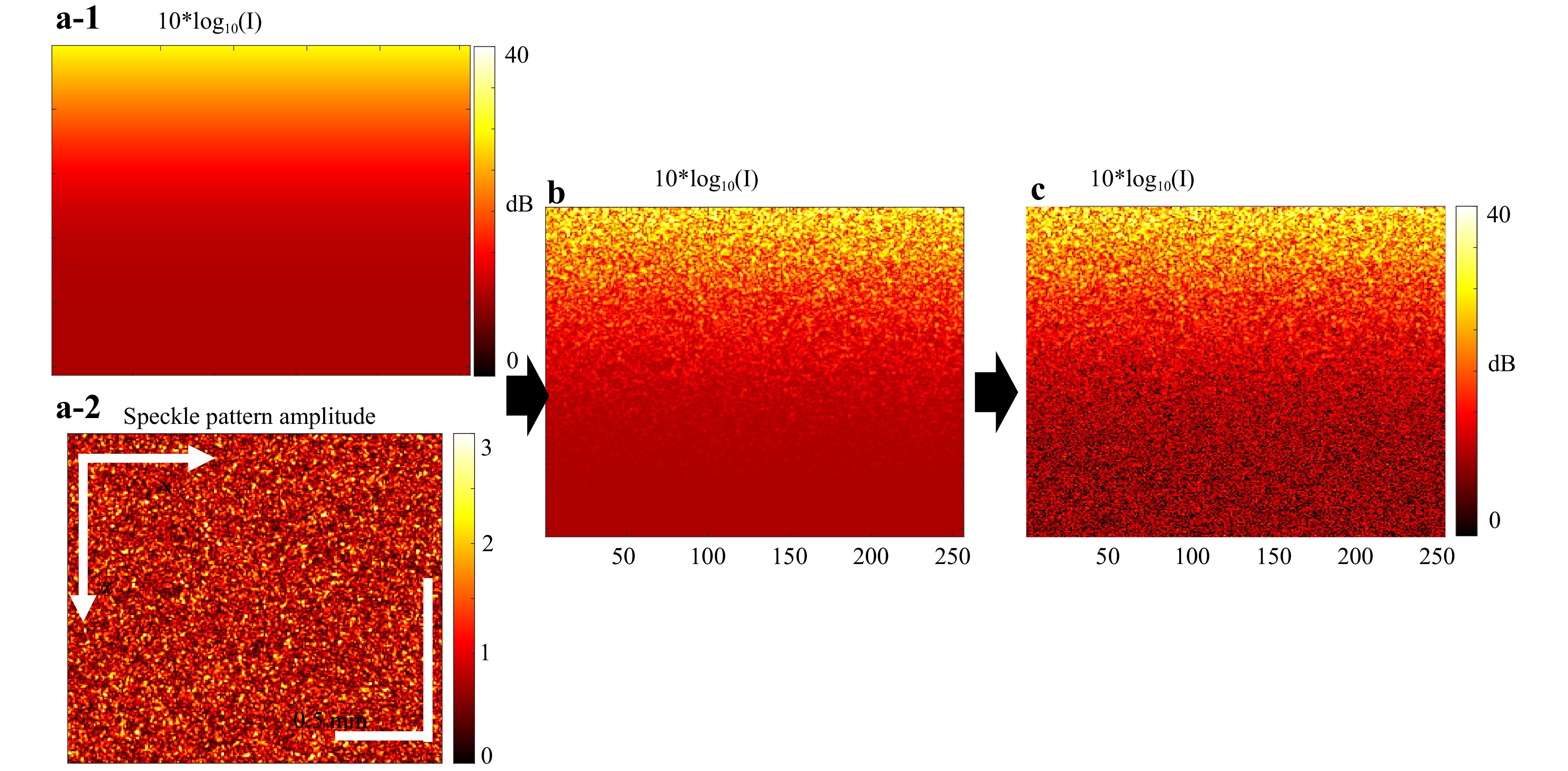
Fig. 3  Illustration of naïve approach to simulation of OCT scans with accounting for the scattering-related losses. a-1 is a simulated continuous distribution of the signal-intensity factor given by Eq. 2 for a spatially homogeneous scattering-dominated attenuation coefficient $ {\mu _s} = 5 $mm^−1, and a-2 is the attenuationless structural OCT scan (simulated using approach³³ as described in Section 3.1). b Structural OCT scan obtained by combining the attenuation-less speckle pattern a-2 with the continuous attenuation factor a-1 and represented in a logarithmic scale. c is the simulated B-scan obtained from b by adding a random complex-valued Gaussian quantity in each pixel to imitate additive measurement noise.

For simple imitation of optical signal attenuation, in most biological tissues, the OCT signal attenuation is dominated by scattering rather than absorption³⁶. Consequently, the optical intensity decay may be characterised by the coefficient $ {\mu _s} $—the optical attenuation coefficient (OAC), entirely determined by scattering. Following Ref. 37, we note that Eq. 1 generates a complex-valued amplitude (with both amplitude and phase). Therefore, to obtain the corresponding intensity, the complex-valued scan must be pixel-by-pixel multiplied by its complex-conjugate value. Thus, in the resulting intensity image, for a chosen desired distribution of $ {\mu _s} $ as a function of the depth coordinate, the signal intensity in the q-th pixel $ {I_0}({{\textit z}_q}) $ in an A-scan is determined by the scattering coefficient $ {\mu _s}(q) $ multiplied by the factor describing the attenuation of the optical signal during its forward-and-backwards propagation between the illuminating/receiving aperture and the scattering sample volume:

Thus, the A-scan intensity in the presence of attenuation can be written as

Here, $ I({{\textit z}_q}) $ is the intensity of the q-th pixel in the A-scan and $ {I_0}({{\textit z}_q}) $ can be interpreted as the pixel intensity $ |A_{px}^2(q)| $, where the amplitude $ A_{px}^{}(q) $ is generated using Eq. 1, in which the scattering-related signal attenuation is neglected. The so-obtained scans are shown in Fig. 3. In such a simple manner, OCT scans can be realistically simulated under scattering-dominated attenuation without a detailed consideration of scattering-related signal losses. When attenuation is introduced in a complex-valued scan, its pixel amplitudes should be multiplied by the square root of Eq. 2. The platform configuration used in this study required approximately 6 min. to generate a “typical” B-scan of 256 × 256 pixels with 64000 scatterers, which is comparable with the spatial density of biological cells and enables fully developed speckles³², as illustrated in Fig. 3 (the generation time is linearly proportional to the number of scatterers and the number of required A-scans).

In this section, following Ref. 38, we outline a more accurate account of scattering-related signal decay, which can be achieved by considering the signal intensity loss at each act of illuminating-beam scattering on individual localised scatterers. The portion of power lost at each scattering event is proportional to the intensity of the incident wave and the scattering cross-section of each scatterer. This portion of the scattered power should be subtracted from the total power of the beam, such that the beam intensity gradually decays with increasing depth. We also consider that the optical signal experiences attenuation in equal proportions during the forward and backward propagation paths.

Based on the assumption that optical attenuation in turbid biological tissues is dominated by energy losses due to scattering, the wave amplitude $ A_j^{rcv} $ received from the j-th scatterer can be written as

where $ \alpha $ characterises the receiver sensitivity, function $ B({x_j},{y_j}) $ corresponds to the lateral amplitude profile, normalised to unity for a given A-scan at the upper boundary of the tissue (usually, this is a Gaussian profile), parameter $ {L_j} \leqslant 1 $ characterises the attenuation of the intensity of the beam propagated from the source to the j-th scatterer, and $ {P_j}^2 $ is the ratio of the beam energy backscattered by the j-th scatterer to the total beam energy at the depth $ {{\textit z}_j} $ corresponding to the j-th scatterer. The latter ratio is proportional to the scattering strength of the j-th scatterer with lateral coordinates (x_j, y_j).

We also assume that the indexes j of the scatterers located within the considered A-scan are sorted in the direction of increasing depth. Thus, taking into account that total attenuation $ {L_j} $ is determined by the energy scattering by all scatterers located above the scatterer with axial coordinate $ {{\textit z}_j} $, the quantity $ {L_j} $ can be expressed in a recurrent form relating it to factor $ {L_{j - 1}} $ describing the cumulative energy loss by depth $ {{\textit z}_{j - 1}} $ of the $ (j - 1) $-th scatterer and parameter $ {P_{j - 1}}^{} $ describing the energy portion back-scattered by the ($ j - 1 $)-th scatterer:

This recurrent expression is valid for indices $ j \geqslant 1 $ and for the initial index $ j = 1 $, the initial values are $ {L_0} $ = 1 and $ {P_0} $ = 0.

The amplitudes $ A_j^{rcv} $ described by expressions (4) and (5) can be substituted into (1) to simulate OCT scans in which the scattering-dominated optical signal attenuation is considered for arbitrary ensembles of scatterers with positions $ ({x_j},{y_j},{{\textit z}_j}) $ within the simulated tissue volume. Eqs. 4, 5 complement Eq. 1 and allow the simulation of A-scans by considering the optical energy losses and retaining the simplicity of the model^32,33 describing the OCT scan formation.

The described model utilises the main OCT device parameters (central wavelength, scanning area size, and resolution volume size), a list of scatterer coordinates, $ ({x_j},{y_j},{{\textit z}_j}) $, and their effective scattering cross-sections as inputs. As an output, the model generates an OCT scan representing the complex amplitudes of individual pixels, considering the resultant intensity decay.

The aforementioned approach to OCT scan simulation was also realised as part of the described online platform.

This approach is presented in detail in the literature^39,40 and is briefly summarised here. This requires the rigorous calculation of wavefronts and complex-valued amplitudes of pixels in a B-scan formed by plane-parallel scanning of the illuminating beam with lateral coordinates (x₀, y₀). The beam profile $ {U_L}(x,y;k) $ can be characterised by its angular (transverse) spectrum at the output/receiving aperture:

The spectrum $ g({k_x},{k_y},k) $ can be readily determined numerically for an arbitrary (not necessarily Gaussian) beam profile (see Fig. 4).

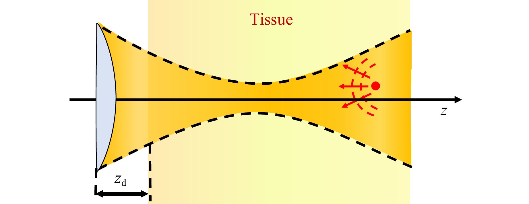
Fig. 4  Schematic of the wave propagation for an arbitrary beam profile.

In spectral form, the wave spectrum incident on the sth scatterer can be written as

where, for the subsequent numerical evaluation, the propagator function can be written in a full non-paraxial form:

where $ {{\textit z}_d} $ denotes the axial coordinates of the lens aperture. In the spatial domain, the wave amplitude $ U_s^{}({x_0},{y_0};k) $ incident on the s-th scatterer can be determined using the inverse Fourier transform of Eq. 7. Thus, the amplitude of the signal collected at the lens aperture after backscattering from the s-th scatterer with scattering strength $ {K_s} $ is given by

As reported in the literature, Eq. 10 can be written in the compact form^39,40

Subsequently, by analogy with Eq. 1, the complex-valued amplitudes of the pixels in each A-scan can be obtained by numerically performing an inverse digital Fourier transform of the spectral amplitudes $ {B_s}({x_0},{y_0};k = {k_n}) $:

Furthermore, research has shown⁴⁰ that if a three-dimensional (3D) set of complex-valued amplitudes $ A\left( {{x_0},{y_0},{{\textit z}_q}} \right) $ is acquired for an initial beam profile $ {U_L}(x,y;k) $, it can be digitally transformed into another form of 3D data corresponding to a target beam profile $ U_L^{(T)}(x,y;k) $. Recalling that the spectral components $ k = {k_n} $ are localised near the central wavenumber $ k = {k_0} $, the expression for the target A-scan can be written as⁴⁰:

where the spectral filtering function $ Filt({{\textit z}_q};{k_0},{k_x},{k_y}) $ is given by

where function $ I({{\textit z}_s};k,{k_x},{k_y}) $ for the initial beam form is

and $ I_{}^{(T)}({{\textit z}_s};k,{k_x},{k_y}) $ is expressed by a similar integral via the target beam angular spectrum $ {g^{(T)}}({k_x},{k_y},k) $. These equations, in the case of OCT scans formed by a highly focused beam (with and without digital refocusing), will be used in Section 5.3 when demonstrating platform usage for mapping speckle contrast.

In this section, we introduce some approaches that are realised on the described online platform and are intended for multimodal processing of OCT scans.

The procedures for phase-sensitive estimation of the axial strain are based on the vector method⁴¹. In this method, the phase-sensitive OCT signals in a pixel with axial index m and lateral index j are characterised by complex-valued amplitudes $ a(m,j) = A(m,j)\exp [i \cdot \varphi (m,j)] $. Until the final processing step, the vector method manipulates signals in complex-valued forms without explicit phase extraction. The main steps of the axial strain estimation in the vector method are as follows.

a) The first step is pixel-by-pixel multiplication of the deformed B-scan and the complex-conjugate initial (reference) scan:

Here, $ \Phi (m,j) = {\phi _2}(m,j) - {\phi _1}(m,j) $ and $ B(m,j) = {A_2}(m,j){A_1}(m,j) $.

b) At the second step, vector averaging of the matrix $ b(m,j) $ is performed using a small sliding window $ {W_z} \times {W_x} $ pixels in size (in practice, 2-3 pixels may suffice):

c) To determine the axial phase variation gradients, the following matrix must be calculated:

It contains the phase difference $ {\Psi _{}}(m,j) $ between the pixels with axial indices $ m $ and $ m + g $, where the interpixel distance $ g $ is the step over which the phase variation gradient is estimated.

d) To further suppress noise, vector averaging of the quantity $ d(m,j) $ can be used with a window of size $ M \times J $ pixels.

The window size $ M \times J $ in Eq. 18 is determined by the desirable resolution of the reconstructed strain field and is typically significantly larger than $ {W_{\textit z}} \times {W_x} $ in Eq. 16, because the scale of spatial variation in the gradient $ {\Psi _{}}(m,j) $ is usually much larger than the scale of variation in the interframe phase difference $ \Phi (m,j) $.

e) The estimated strain is expressed via the phase-difference gradient $ {\hat \Psi _{}}(m,j) $ as

where $ {k_0} = 2{\text π} /{\lambda _o} $ is the central wavenumber of the OCT source spectrum in vacuum and $ {h_{\textit z}} $ is the axial distance between the centres of adjacent pixels in vacuum.

As described in Ref. 42, such procedures of strain estimation may then be used to estimate the elasticity of tissues using a comparison of strains in the tissue and reference translucent layer (usually made of silicone).

In the abovementioned variant of the vector method based on Ref. 41, the optimal selection of averaging-window sizes and the scale $ g $ used for estimating the phase-variation gradient was not addressed. With appropriately chosen averaging-window sizes and gradient-estimation scales, the vector method demonstrates exceptional robustness with respect to various measurement noises, as demonstrated in Ref. 41 in which the processing parameters were fixed. The procedures for the adaptive selection of the gradient-estimation scale and averaging-window sizes were specifically discussed in Refs. 43−45, which is especially important for the reconstruction of strains exhibiting pronounced spatial and temporal variability typical of real tissues. Another advantage of the strain-estimation method⁴⁶ based on the least-squares estimation of interframe phase-variation gradients is that the described vector method does not require phase unwrapping and is significantly faster computationally, as highlighted in Ref. 42.

Another modality realised in the proposed platform is the spatially resolved estimation of the OAC $ {\mu _s}({\textit z}) $. The OAC can be derived from Eq. 3 as described in ref. 36 Briefly, in the absence of additive measurement noises and in the case of complete decay of the observed signal intensity $ I({\textit z}) $ within the visualised region, for an arbitrary form of $ {\mu _s}({\textit z}) $, the following rigorously valid expression was derived in³⁶

Physically, Eq. 20 reflects the fact that the optical beam energy passing through the depth coordinate $ {\textit z} $ is equal to the energy loss caused by scattering during optical beam propagation from the current depth $ {\textit z} $ to an infinite depth.

Note that Eq. 22 is written in the continuous form and is rigorously valid only at semi-infinite intervals. However, OCT scans are always acquired using a finite depth interval $ {\textit z} \leqslant H $ and have a pixelated form. Therefore, the discretised counterpart of Eq. 20 can be written as follows:

where $ {I_j} $ is the intensity of the OCT signal in the j-th pixel and $ \Delta {{\textit z}_{px}} $ is the axial pixel size for normalisation of the depth-resolved attenuation coefficient $ {\mu _n} $ estimated for n-th pixel in the depth direction, where index n = 1 corresponds to the surface. Here, we assume that in the pixel with the maximum index $ N $, the intensity $ {I_N} $ tends to zero.

The commonly calculated parameter characterising speckles in OCT images is the normalised speckle contrast (SC) parameter defined for the intensities of speckels^38,47,48:

where I is the intensity of the OCT signal at each pixel within the processing window used for SC estimation, the operator $ \left\langle {} \right\rangle $ denotes the procedure of pixel intensity averaging within the chosen processing window, and $ \sigma $ is the standard deviation of the intensity within this window. We recall that speckle contrast is expected to tend towards unity $ {\sigma _I} \to 1 $ for a homogeneous scatterer distribution with a high scatterer concentration (with a few or more scatterers in each sample (coherence) volume of the OCT beam)⁴⁸. For small scatterer concentrations (less than unity in each sample volume) or strong spatial inhomogeneities in the scatterer distribution in the selected window, the speckle contrast exhibits spikes, $ {\sigma _I} \gt > 1 $.

As shown in Ref. 38, the SC value is affected by signal attenuation in the depth direction. This attenuation produces an additional inhomogeneity pattern which increases the SC value. This also creates a confusing correlation between OAC and SC. Therefore, to eliminate the attenuation-induced interrelation between SC and OAC, we compensated for signal attenuation using an OAC-based approach prior to the calculation of SC for the corrected intensity of speckles:

where $ {I_{0q}} $ is the uncorrected pixel intensity, $ {I_q} $ is the corrected pixel intensity, $ q $ is the pixel index corresponding to the current depth, and index $ N $ corresponds to the maximal depth.

For polarisation-sensitive devices, such as OCT 1300 produced at IAP RAS, in which OCT images are formed for two channels, co-polarisation and cross-polarisation, one may estimate the depolarisation ratio, which is defined as the ratio of the signal intensities in the cross- and co-polarisation channels:

where $ \left\langle {} \right\rangle $ refers to the averaging over a chosen sliding window. The calculation of this quantity was implemented on the described online platform.

In this section, we focus on tuning and testing the above described signal analysis procedures using digital phantoms which may also be generated using the tools for OCT-data simulations implemented in the decribed platform.

The described approach to OCT signal simulation readily allows the generation of sequences of OCT scans in which any desirable interframe displacements of the scatterers can be introduced. To imitate tissue straining, we simulated scans for some initial positions of the scatterers and then for strain-induced displaced positions of the scatterers (e.g. produced by tissue compression). In the simulations, the displacements of the scatterers (1024 for each A-scan consisting of 256 pixels) with random initial coordinates corresponded to the prescribed strain distribution shown in Fig. 5b. Fig. 5c shows the corresponding colour map of the inter-frame phase variations, demonstrating pronounced lateral inhomogeneity. Fig. 5 illustrates the reconstruction of interframe strain distribution using the “vector” method (see Section 4.1) in which the complex-valued amplitudes are treated as vectors in the complex plane without explicit utilisation of phase till the final processing step. The simulation parameters in Fig. 5 correspond to an OCT system with a central wavelength of 1300 nm, a spectral width of 90 nm, and an A-scan depth of 2 mm in air, corresponding to 256 pixels.

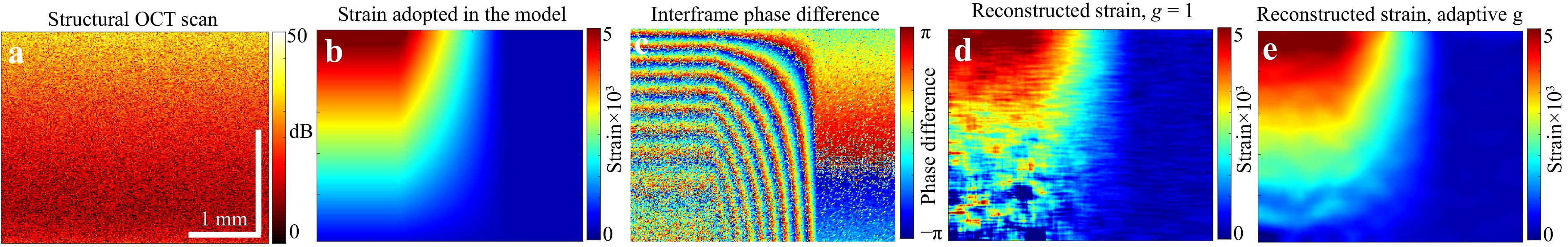
Fig. 5  Simulation results for the case of inhomogeneous strain field. a is the structural image; b the interframe strain distribution adopted in the model; c is the corresponding color map for interframe phase difference; d reconstructed strain map using the vector method⁴¹ with a fixed small scale $ g = 1 $ used for phase-gradient estimation; e is the strain map reconstructed using the vector method with adaptive choice of the gradient-estimation scale $ g $ following ref. 43, which efficiently reduces the errors in the in the strain estimation.

The preliminary testing of phase-sensitive strain mapping on digital phantoms is useful for the development of compression OCE which are widely used in various biomedical applications⁴².

Various OCT-based approaches for reconstructing OAC parameters have attracted considerable attention in recent years³⁶. Comparative testing of such methods under highly controllable conditions is crucial to understand their operability and accuracy in real applications. The application of digital phantoms for such tests was discussed in a recent paper³⁷. An example illustrating the masking role of the “speckle noise” intrinsic to OCT scans is given in Fig. 6. The initial B-scan was simulated as described in Section 3.1, and the scattering-related attenuation was introduced as described in Section 3.2. The assumed OAC distribution $ {\mu _s}({\textit z}) $ is shown in Fig. 6a-1, and the corresponding structural OCT scan is presented in Fig. 6a-2. From left to right, intensity image 6(a-2) represents four vertical columns corresponding to the $ {\mu _s}({\textit z}) $ layers shown in Fig. 6a-1 and found for the following conditions: (I) Noiseless intensity distribution continuously reconstructed from $ {\mu _s}({\textit z}) $ via Eq. 2; (II) the same data as in (I) but with additive measurement noise; and (III) is based on a combination of additive noise and the simulated OCT scan formed as described in Section 3.2, combining the desired continuous distribution $ {\mu _s}({\textit z}) $ of the optical scattering parameter and the initial OCT scan in which the speckle structure is simulated via Eq. 1 neglecting the scattering losses; (IV) is similar to column (III) but in the absence of additive noise. In all cases, the method³⁶ was used to perform spatially resolved OAC mapping. Initially, this estimation was performed without spatial averaging, as shown in Fig. 6b-2. Without averaging, the speckle noise nearly completely masked the assumed regular distribution of the OAC. Subsequently, averaging was applied over rectangular windows of 10 × 10 pixels (Fig. 6c-2) and 20 × 20 pixels (Fig. 6d-2). Averaging over the sliding window $ {W_I} $ was initially performed for the initial intensity scan, and then the $ {\mu _s} $ values that were estimated using the method³⁶ were additionally averaged over the sliding window $ {W_{{\mu _s}}} $ with the same size as for $ {W_I} $. The window sizes are shown in figure.

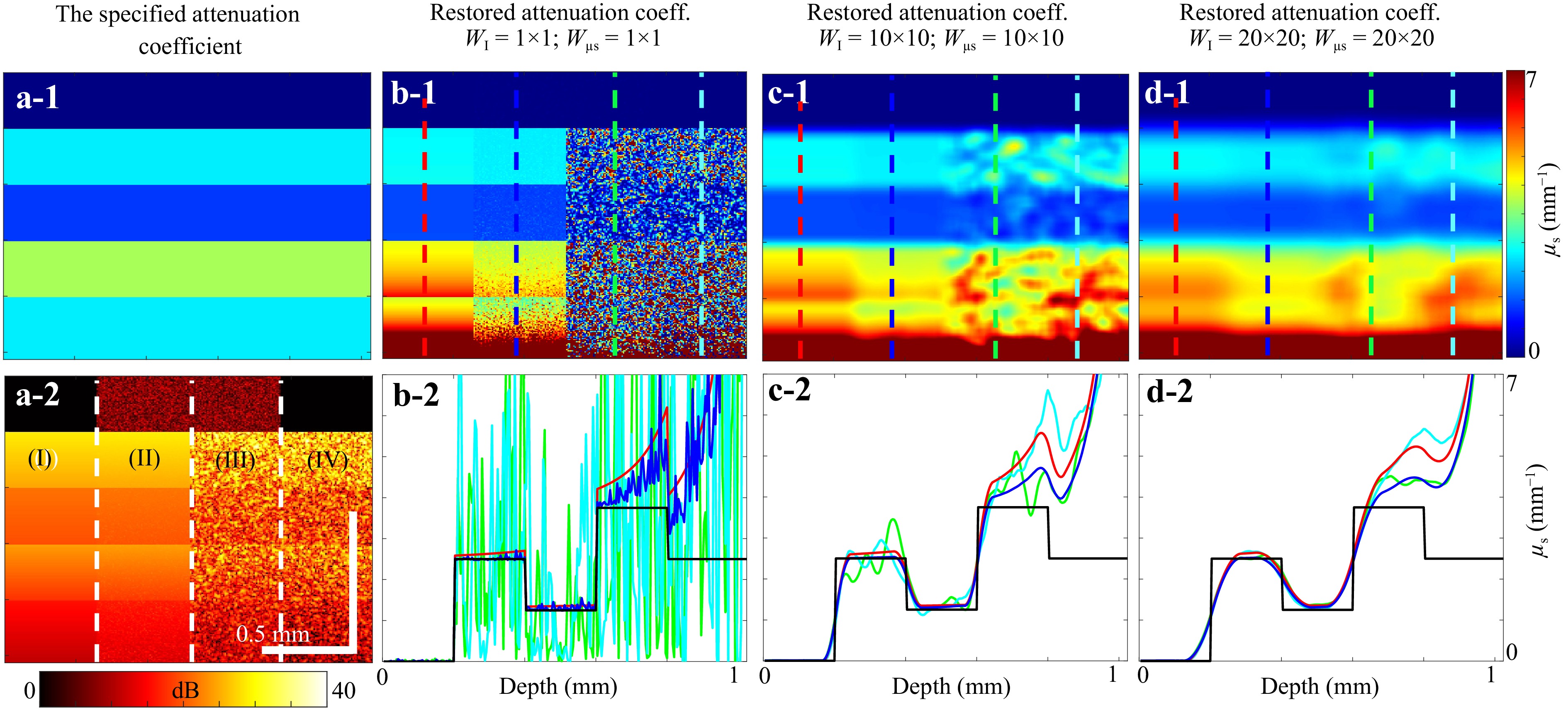
Fig. 6  Demonstration of OAC reconstruction following ref. 37 for several variants of preliminary averaging of intensity scans and subsequent averaging of reconstructed $ {\mu _s}({\textit z}) $ using sliding windows 1 × 1, 5 × 5, and 20 × 20 pixels. a-1 distribution of OAC adopted in the model. a-2 the corresponding simulated structural OCT scans with sub-regions (I)-(IV) with various combinations of the speckle noise and additive measurement noises as explained in the text. b-1, c-1 and d-1 reconstructed OAC maps using the averaging windows with the sizes indicated above the plots for the same regions (I) – (IV) that are shown in a-2. Panels b-2, c-2 and d-2 vertical profiles of the reconstructed OAC; the colors of the curves showing the reconstructed OAC profiles correspond to the colors of vertical dashed lines in panels b-1 – d-1, along which the OAC profiles were estimated.

Note that the reconstructed OAC demonstrates an artefactual increase closer to the maximal imaging depth. This artefactual effect is intrinsic to the method³⁶ and is caused by insufficiently strong decay of the OCT signal within the visualised depths. Various studies have aimed to mitigate this artefactual effect; for example, Ref. 49. The described platform enables a convenient means of simulating diverse, highly controllable scenarios of OAC distribution, such that various approaches may be comparatively tested.

The described approach for the generation of digital phantoms can also be used to evaluate various effects that influence speckle contrast values. As an example, we present simulation data for uniform in average random distribution of scatterers and a pronouncedly focused illumination beam. Focusing may pronouncedly change the size of the sample volume such that near the focus and beyond the focus, the sample volumes may contain significantly different amounts of scatterers. Here, the “sample volume” is conventionally defined as a cylindrical volume with the lateral size determined by the beam cross section and the axial size equal to one-half of the coherence length. In particular, when the sample volume contains at least several scatterers, the situation corresponds to well-developed speckles, for which the speckle contrast parameter SC, defined by Eq. 22 is expected to be close to unity, $ SC \to 1 $. However, it may happen that for a strongly focused illuminating beam, the speckles may be well developed only beyond the focal region. However in the focal region, where the beam diameter is several times smaller, the number of contained scatterers is also smaller, so that the speckles in the focal regions are not yet fully developed. Consequently, an elevated value of speckle contrast should be expected in this region.

This situation, illustrated in Fig. 7, was simulated using Eqs. 6–11 for a strongly focused OCT beam and spatially homogeneous distribution of scatterers. Fig. 7a-1 shows the resultant structural scan, demonstrating that near the focus depth, the scatterers appear brighter; however, their spatial distribution appears somewhat sparse compared with the regions outside the focal depth, where the illuminating beam diameter is several times greater than that in the focus. Fig. 7a-2 shows the depth dependence of the speckle contrast parameter determined using Eq. 22. This plot shows that beyond the focal region, where each sample volume contains at least several scatterers, the speckles are fully developed and the speckle contrast parameter is close to unity. However, as explained above, in the focal region, the sample volume is several times smaller and contains several times smaller amount of scatterers. Consequently, the speckles are underdeveloped, and the speckle contrast parameter is elevated (in this example, $ SC \sim 2 $).

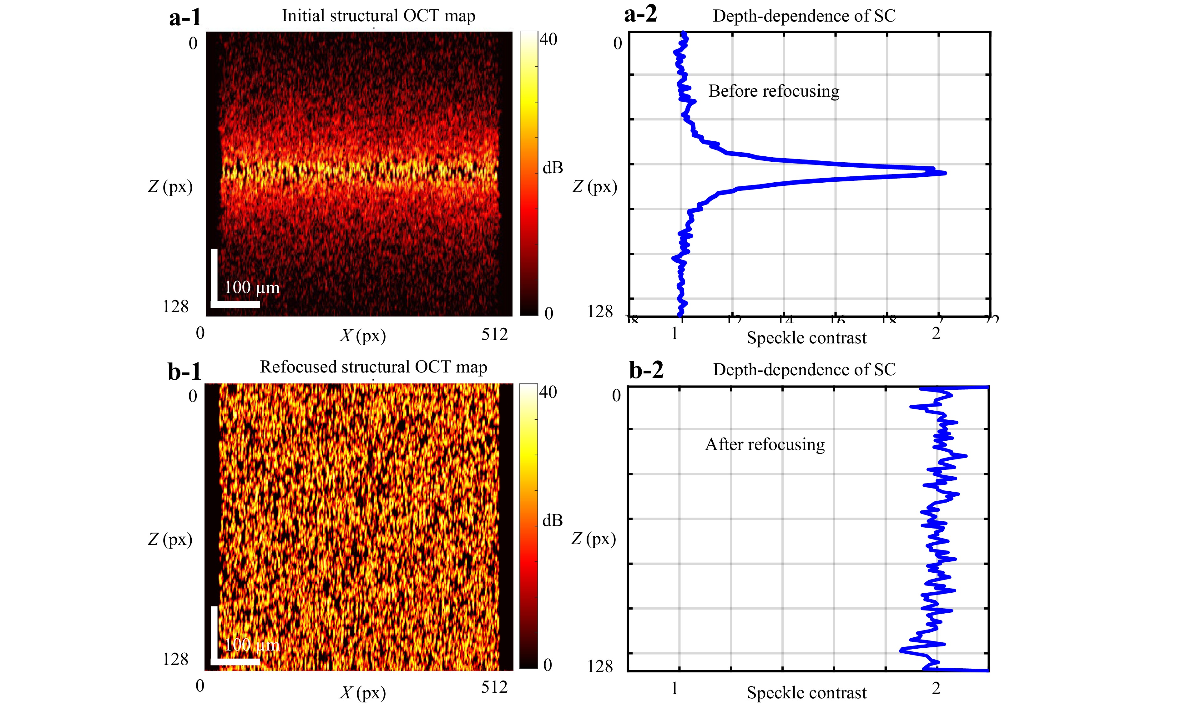
Fig. 7  Influence of the degree of illuminating-beam focusing on the estimated speckle contrast. a-1 Simulated B-scan for a uniform spatial distribution of scatterers under a highly focused illuminating beam; a-2 Depth-dependence of the estimated speckle contrast, demonstrating speckle contrast (SC) value ≈ 1 outside the focal region and approximately twice that value near the focus. b-1 Refocused structural scan. b-2 Corresponding estimated SC-parameter which becomes nearly depth-independent and close to SC ≈ 2 at the physical focus. In this example, the focal-spot radius is 1.9 μm, the central wavelength is 0.85 μm and the Rayleigh length is approximately 13 μm, yielding a total axial focal-waist length of 26 μm.

Furthermore, if a sufficiently densely recorded 3D set of complex-valued OCT data is available, these data can be digitally refocused, for example, by applying the K-space approach⁴⁰ outlined in Section 3.4. The resultant refocused structural OCT scan is shown in Fig. 7b-1, for which the effective size of the sample volume is approximately the same as that of the physical focus in Fig. 7a-1. Consequently, the speckle contrast parameter for the refocused data becomes depth-independent and close to the value of $ SC\sim 2 $ in the physical focus.

In this section, we provide examples of practical applications of the presented no-code OCT software platform in the context of cancer tissue evaluation. By leveraging multimodal OCT signal processing techniques, the platform demonstrated the high-contrast differentiation of tumourous and non-tumourous regions in various cancerous tissues. Platform-based processing of real OCT signals comprises imaging techniques, such as optical attenuation imaging, speckle contrast imaging, depolarisation-ratio imaging, strain imaging, and elastographic (tissue stiffness) imaging. We illustrate these applications with case studies involving the brain, skin, and endometrial tissues, highlighting the capability of the platform to visualise tumour margins.

This example relates to the analysis of a patient’s brain tissue B-scans obtained intraoperatively during surgical operations aimed at excising malignant tumours. The upper row in Fig. 8 shows the initial co-polarisation structural scan (panel (a)), cross-polarisation structural scan (b), and histological image (c) obtained by histopathology post-surgery, such that the direction of cutting the histological slide only approximately corresponded to the orientation of the OCT B-scans directed to the brain tissue depth. The lower row in Fig. 8 presents the derived attenuation map (d), speckle contrast map (e), and depolarisation ratio map (f). The structural copolarisation OCT scans demonstrated minimal differences between the images. In the cross-polarisation scan, the signal level is relatively brighter on the right-hand side, corresponding to normal tissue; however, the difference from the tumour region is still not clear.

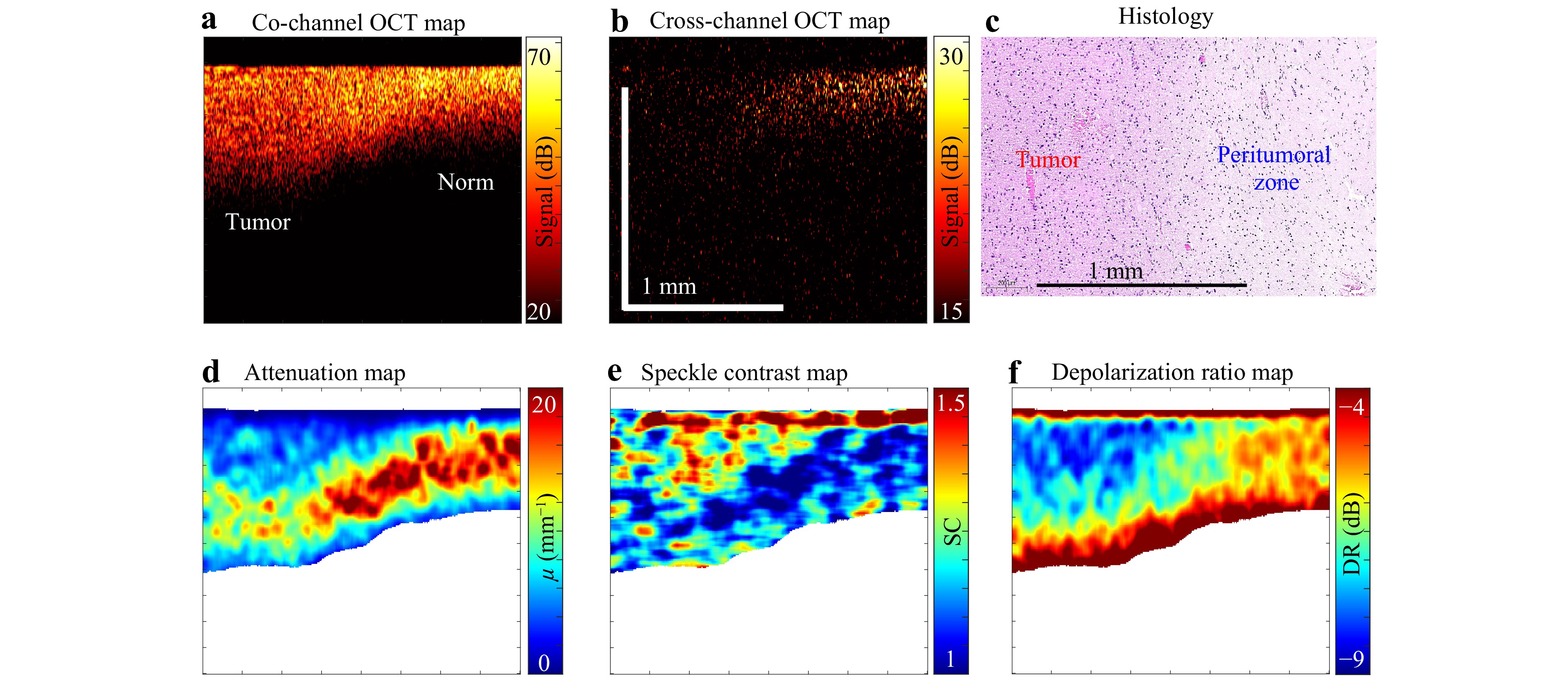
Fig. 8  Application of the multimodal OCT imaging to cancerous brain tissue. a Initial co-polarisation OCT scan; b cross-polarisation OCT scan; c histological image approximately co-located with the OCT scans. The lower row presents the derived maps: d optical attenuation, e speckle contrast, and f depolarisation ratio, determined as described in the literature⁵⁰. In these derived maps, the contrast between the left and right halves—corresponding to tumour and non-tumour regions—is substantially higher than in the initial OCT images.

The examples in Fig. 8 qualitatively demonstrate a much higher contrast between normal and timorous tissues in the derived maps of the OCT scan characteristics in comparison with the initial structural scans. A recent paper⁵¹ presented discussions of quantitative formulations and the performance of diagnostic criteria based on the combined use of optical attenuation and speckle contrast for the differentiation of three medically important brain tissue classes: (i) malignant, (ii) damaged but not yet malignant, and (iii) normal brain tissue.

This section presents an example of multimodal processing of 3D OCT data sets acquired from patient-derived xenograft cell-line of pancreatic cancer grown in mice dorsal skinfold window chambers, similar to a previous study⁵². The results are shown in Fig. 9, where panel (a) shows an en-face structural image of the tumour and peritumoural zone corresponding to the depth z = 200μm, whereas panel (b) is a similar en-face view but with averaging over the depth interval [175, 225] μm. In this study, in addition to OCT imaging, the tumour zone was visualised by a fluorescence label, which enabled differentiation between the tumour and peritumoural tissues. Furthermore, by registering a series of 24 repeated scans at each B-scan position, the blood vessels were visualised using the speckle-variance principle⁵³. The tumour region was contrasted by fluorescence imaging (similar to a previous study⁵⁴), and the fluorescence-contrasted zone of the tumour location served as the ground truth for comparison with other contrast modalities based on OCT-scan analysis, as shown in Fig. 9. Panel (c) in Fig. 9 shows an en-face speckle-variance-based angiographic image superposed with the fluorescence-based image of the tumour tissue in the central part of the panel. Panel (e) shows the same fluorescence-contrasted tumour zone superposed with the en-face speckle contrast image plotted with averaging over the same depth interval as the structural image in panel (b). The central tumour zone of dark-blue color corresponding to $ SC \approx 1 $ in panel (e) perfectly matches the fluorescence-based image of the tumour tissue. The next panel (f) shows a similarly depth-averaged optical-attenuation map also superposed with the fluorescence-contrasted image of the tupor tissue. Panel (f) indicates that in the central part of the tumour, the attenuation demonstrates elevated values, whereas in the narrow zone of the tumour periphery, the attenuation is significantly reduced and then gradually increases again in the peritumoural regions.

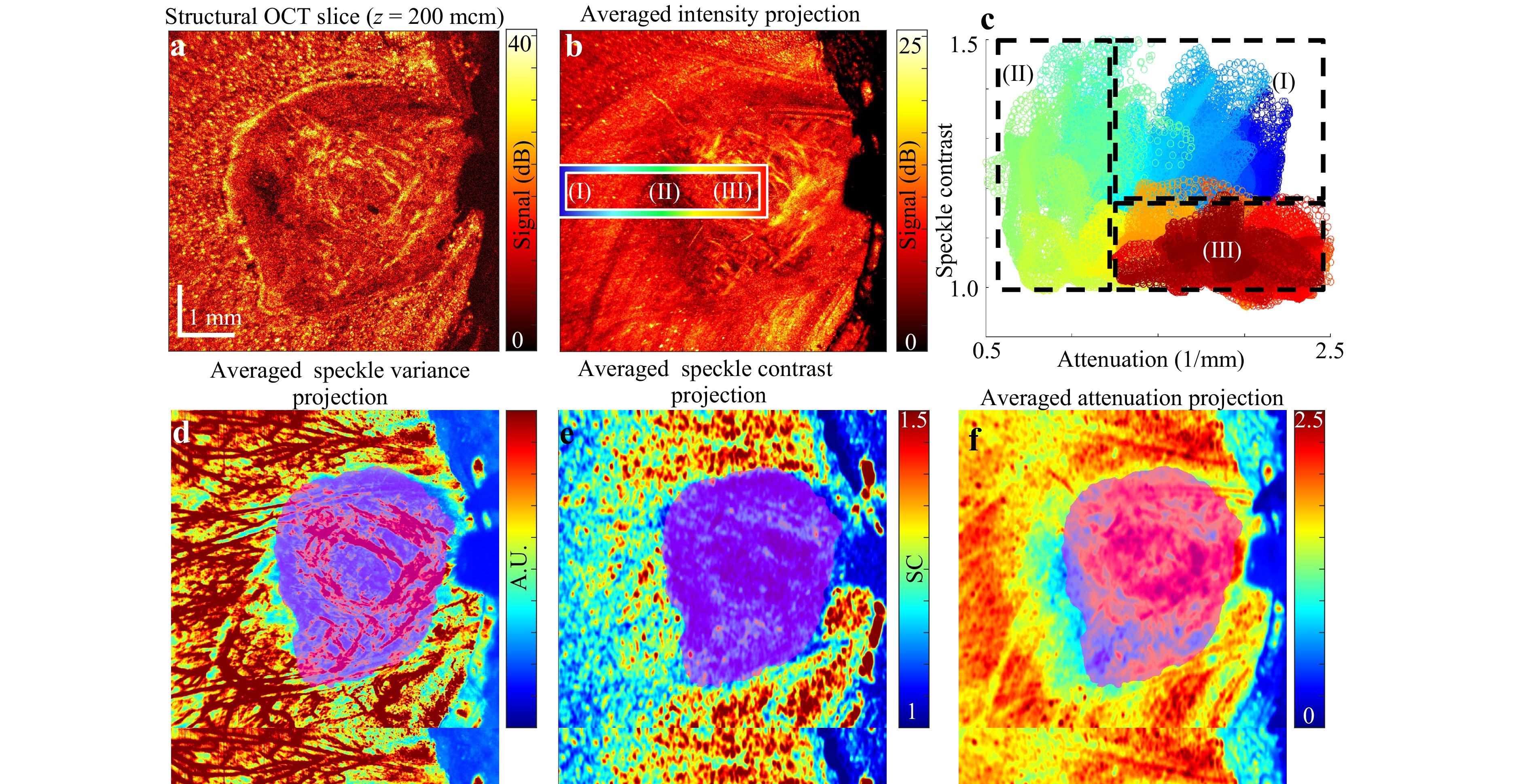
Fig. 9  Application of the multimodal OCT to murine cancer imaging. a En-face structural OCT image corresponding to a depth of z = 200 μm. b En-face intensity image averaged over the depth range [175, 225] μm. d Speckle-variance-based en-face angiographic image superposed with the fluorescence-contrasted visualisation of the tumour’s central region. e Speckle contrast map averaged over the same depth range as in b, showing excellent agreement with the superposed fluorescence-contrasted image of the tumour core. f Optical attenuation map averaged within the same depth range as in b and e, also superposed with the fluorescence-contrasted visualisation of the tumour centre. c Two-dimensional plot of attenuation versus speckle contrast, where each point represents a pixel from the rectangular region marked in b. Colours in c denote positions within this region, progressing from subregion I (blue) through subregion II (green) to subregion III (red).

A useful representation of the possibility of differentiating the peritumoural zone, tumour boundary, and tumourous tissue itself can be obtained from panel (c) of Fig. 9. This is a 2D plot of the plane (attenuation and speckle contrast). The plot corresponds to the pixels located within the rectangular zone shown in Fig. 9b, where subregion (I) corresponds to the peritumoural zone, (II) is localised near the tumour boundary, and (III) corresponds to the central region of the tumour. The colour of each point in the 2D plot in panel (c) denotes its position, starting from zone I (blue) via zone II (green) to zone III (red). Panel (c) clearly shows that zones I and III demonstrate an elevated attenuation of comparable magnitudes, whereas the speckle contrast parameter in zone I is higher than that in zone III. In contrast, zone II has clearly lower attenuation values than both zones I and III (this fact was already mentioned above); however, the speckle contrast parameter in zone II demonstrates a broad range of values overlapping with the speckle contrast values typical of both zones I and III.

The next example relates to melanoma of the patient’s skin. The OCT device used in these examinations enabled only a copolarisation channel. However, unlike the B-scans of the patient’s brain in Section 6.1, 3D datasets are available in this example. Fig. 10a-1 shows the en-face OCT image for a depth of z = 33 pixels (the vertical pixel size is approximately 7 μm), in which the region of normal tissue corresponds to the upper-right corner. Two vertical dashed lines (the left line passes mostly through the cancerous zone, and the right line passes mostly through the normal tissue) correspond to the positions of the OCT B-scans shown in Fig. 10a-2 (for normal) and Fig. 10a-3 (for tumour zone). Panels (b-1), (b-2), and (b-3) in Fig. 10 show the derived attenuation maps corresponding to OCT scans (a-1), (a-2), and (a-3). In Fig. 10b-1, also obtained for z = 33 px, as in Fig. 10a-1, the tumour zone exhibits elevated values of $ {\mu _s}\sim 15 - 20 $ mm⁻¹ which are clearly higher than the normal region with approximately twice the values of $ {\mu _s} $. In the vertically oriented attenuation maps in Fig. 10b-2 and Fig. 10b-3, the pronounced vertical inhomogeneity of $ {\mu _s} $ is visible, with clearly different depths and clustering characteristics between the normal and tumour regions.

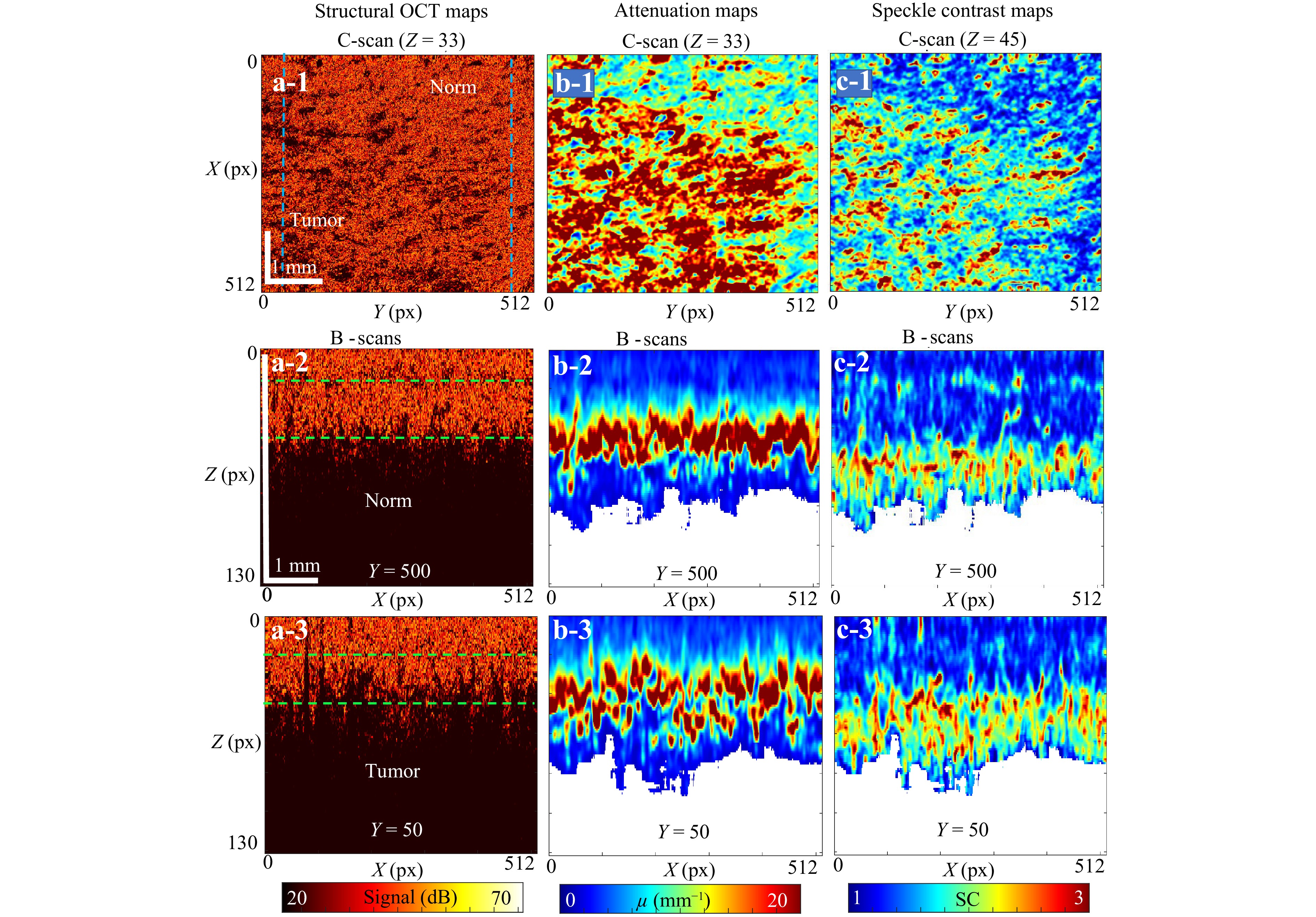
Fig. 10  Application of the multimodal OCT imaging to a melanoma region of patient’s skin. a-1 is the en-face OCT image for a depth of z=33 px depth (the vertical pixel size is about 6 μm). Two vertical dashed lines correspond to the positions of B-scans shown in a-2 for the normal and a-3 tumour regions. Panels b-1, b-2 and b-3 are the derived attenuation maps corresponding to OCT scans a-1, a-2 and a-3, respectively. In b-1 also obtained for z = 33 px like a-1, the tumour zone in Fig. 10 exhibits elevated values of $ {\mu _s}\sim 15 - 20 $ mm⁻¹, whereas the normal region has about twice lower values of $ {\mu _s} $. Panel c-1 shows the en-face speckle contrast maps (for the depth z = 45 px). c-2 and c-3 are the vertically-oriented speckle contrast maps, which demonstrate clearly different depth distributions and different character of clustering in C-scans for the normal and tumour.

The en-face speckle contrast map in Fig. 10c-1 (obtained for depth z = 45 px) also demonstrates the difference between the normal and tumour regions, for which the evaluated values of the speckle contrast parameter are typical. The vertical speckle contrast scans in Fig. 10c-2, 10c-3 demonstrate different depth distributions and different clustering characteristics of speckle contrast values for the normal and tumour regions.

The OCT imaging shown in Fig. 10 was performed in vivo in a region clinically diagnosed as melanoma by an experienced dermatologist through visual examination. The structural OCT scans revealed only subtle texture differences between normal skin and the suspected melanoma, leading to a recommendation for surgical excision. Post-excision histology confirmed the diagnosis, although precise co-location of histological images with the in vivo OCT scans was challenging. Post-processed OCT data presented in Fig. 10 reveal that the contrast between malignant and normal tissues in the derived optical attenuation and speckle contrast maps is markedly enhanced compared with the structural images. A related medical application of this processing approach involves assessing variations in skin layer thickness across different regions. Mapping optical attenuation and speckle contrast can therefore support direct skin-layer segmentation or serve as an annotation tool for developing machine-learning-based segmentation methods⁵⁵. Overall, advanced skin scan processing substantially enhances the diagnostic value of OCT by providing clinicians with objective, quantitative information.

In this section we demonstrate the application of strain mapping for realization of compression OCT elastography. This realization is based on utilization of pre-calibrated translucent silicone layers placed on the surface of the examined tissue. , During compression by the OCT probe, the strain was simultaneously estimated in the reference silicone and examined tissue. In both silicone and tissue the compression-induced strain was found via the interframe phase variations using the vector method as described in Section 4.1. Because silicone exhibits highly linear elastic behaviour^56,57, plotting the strain in the silicone versus the strain in the underlying tissue yields spatially resolved dependences of stress $ \sigma $ on strain $ s $ for the examined tissue⁴². After obtaining the stress-strain dependences $ \sigma (s) $ which are usually pronouncedly nonlinear for most tissues, tangent elastic modulus $ {E_{tg}} = d\sigma /ds $ can be estimated for a pre-selected stress level, so that “stress-standardized” stiffness maps can be plotted⁵⁶.

Fig. 11 illustrates the application of such elastographic OCT imaging to characterise cancerous regions in endometrial tissue. Panel (a) shows the structural image where the reference silicone layer is clearly seen above the studied tissue, in which a slightly brighter region on the right-hand side corresponds to the cancerous region (which is validated by the corresponding histology shown in panel (d)). However, brightness in the structural scans strongly depends on several factors and cannot be used as a reliable diagnostic parameter. Panel (b) shows the attenuation map in which the attenuation parameter is independent of the absolute intensity. However, the difference between the cancer and norm in the attenuation map is not yet sufficiently clear, unlike panel (c), which shows the stiffness map. In the elastographic map, the cancerous tissue region is clearly visualised as a region with strongly elevated stiffness on the right side of panel (c), demonstrating good consistency with the histological image.

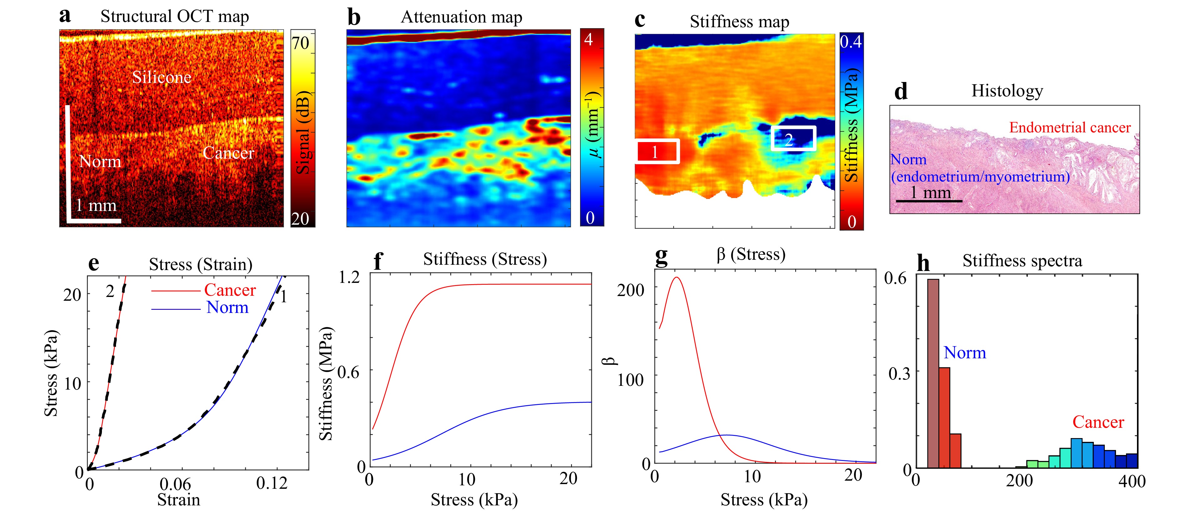
Fig. 11  Application of the multimodal OCT imaging to characterize cancerous regions in endometrial tissue. a is an example of structural image of an endometrium tissue sample with the superposed layer of reference silicone used as an optical stress sensor; b is the derived spatially resolved attenuation map; c is the map of tangent Young’s modulus plotted for 3 kPa applied stress; d is the corresponding histological image demonstrating a good agreement between the zone of endometrial cancer and the zone of strongly elevated stiffness in c. Panel e shows examples of spatially resolved pronouncedly nonlinear stress–strain curves for the normal tissue cancerous tissue (the corresponding regions are indicated in c); the dashed lines in e are experimental and solid ones are the fitting curves; f shows the stress dependences of the tangent Young’s modulus derived from the initial stress–strain curves $ \sigma (s) $; g shows the stress dependences for the dimensionless nonlinearity parameter $ \beta = d{E_{tg}}/d\sigma $; h present the “elasticity spectra” for the zone of normal tissue (smaller stiffness values) and the cancerous tissue (larger stiffness values).

Furthermore, the developed technique enables detailed characterisation of tissue elasticity through the analysis of spatially resolved stress–strain curves. Panel (e) shows two such stress–strain curves obtained for normal and cancerous tissues (for the locations indicated in Fig. 11c). The dashed lines represent the experimental results, and the solid lines represent the fitting curves based on the physically substantiated model⁵⁸ describing tissue nonlinearity. Verification confirmed that this model provides high-quality fitting of nonlinear stress–strain dependencies across a broad range of tissues. Analysis of these fitting curves yields a comprehensive description of the linear and nonlinear elastic properties of the examined tissue. The stress–strain curves shown in Fig. 11e reveal additional dependences, including the dependence of the tangent Young’s modulus (current stiffness) on the stress (Fig. 11f). The tangent modulus $ {E_{tg}} = d\sigma /ds $ usually strongly depends on the applied stress; therefore, its stress sensitivity may be characterised by the dimensionless nonlinearity parameter $ \beta $, defined as $ \beta = d{E_{tg}}/d\sigma $ (Fig. 11g). In some cases, the difference in the tangent Young’s modulus is insufficient for delineation of the examined tissue types; nevertheless, the combined utilisation of the tangent Young’s modulus and the nonlinearity parameter allows the differentiation of such tissue types^59,60_. Spatially resolved estimation of the Young’s modulus further enables comparison of “elasticity spectra” (representing the occurrence frequency of $ {E_{tg}} $ values), as illustrated in Fig. 11h. These elasticity spectra support fine differentiation among various types of cancerous tissue types⁶¹. A detailed discussion of the medical implications and diagnostic accuracy of compression OCT elastography for endometrial cancer and precancer detection, based on strain reconstruction, is reported in a recent publication⁶².

The last example is also based on the strain-mapping tool realized in the described platform. The visualised strain may be of arbitrary origin; therefore, OCT was recently applied to map strains produced by various osmotically active solutions^63,64. For example, these may be solutions of glycerol and other substances which are often used in pharmacology and cosmetics as well as utilised as optical clearing agents to enhance the operability depth of biophotonic-based diagnostic methods^65,66.

Fig. 12 shows the user interface of the online tool used for plotting and analysing the osmotically induced strains. Panels descriptions are provided in the corresponding captions. The realised processing enables detailed analysis of the spatiotemporal dynamics of osmotically induced strain within selected tissue regions, as illustrated in Fig. 12e, f, demonstrating the spatiotemporal dependencies of interframe strains. This form of strain analysis can be considered a variant of OCT elastography, where osmotically induced strains replace mechanical compression (OIS-OCE). An example of the use of such an OIS-OCE for diagnosing the degree of cartilage degradation was recently discussed in Ref. 67. Another application for the characterisation of diffusion kinetics by observing the accompanying osmotic strains is demonstrated in Ref. 68. Additional applications of this OCT-based analysis are anticipated in related biophotonic and diagnostic research domains.

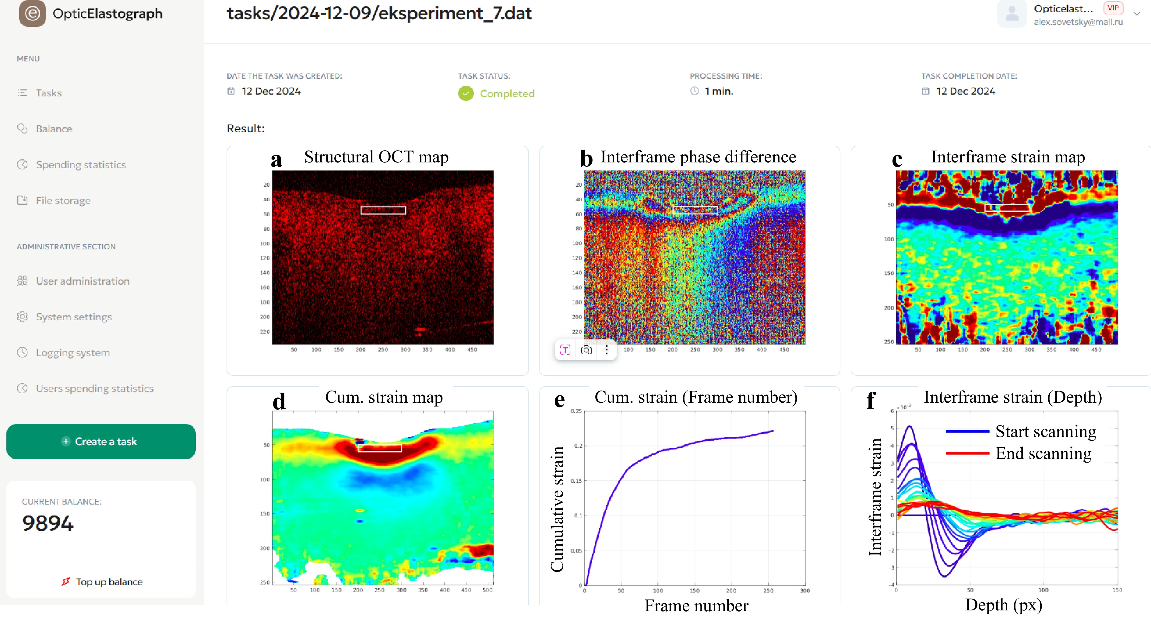
Fig. 12  Application of the multimodal OCT imaging to characterize strains of osmotic origin. This example illustrates strains induced by the penetration of a 30% glycerol solution into the bulk of a cartilaginous sample. The left column shows the menu bar of the online platform, while the other panels demonstrate the results of its application. Panel a presents the structural OCT image; b shows the interframe phase difference caused by osmotically induced tissue straining (obtained for a 1 s interframe interval); c depicts the reconstructed map of osmotically induced interframe strains; d displays the cumulative strain map representing deformation accumulated within the tissue during 260 s after solution application; e illustrates the time evolution of cumulative strain in the tissue expansion zone indicated by rectangles in the preceding panels; and f presents depth profiles of osmotically induced interframe strains recorded at 10 s intervals.

In the previous sections, we outlined the architecture and capabilities of our no-code OCT software platform, which enables realistic wave-based simulations and facilitates the multimodal processing of OCT scans. The platform architecture, which utilises Docker containers to encapsulate Octave code, realises a scalable and reproducible environment for OCT data analysis. This design has proven highly effective in streamlining the development and deployment of OCT signal processing applications across various domains, including oncology.

The wave-based approach implemented in the platform allowed for the simulation of OCT signals under different conditions, such as varying scatterer configurations and device settings. Although the simulations are based on the single-scattering approximation and exclude multiple scattering, this ballistic single-scattering model reflects the fundamental principle of OCT imaging. From a practical viewpoint, our methodology (supported by the results in Refs. 33,34,39,40) offers significant advantages in terms of computational efficiency and the ability to model arbitrary interframe motions of scatterers, a capability essential for the development of elastographic and angiographic OCT methods.

The abovementioned models of OCT signal formation enable the generation of digital phantoms that serve as powerful tools for developing and testing OCT-based diagnostic modalities. These simulations provide a valuable alternative to physical experiments, which can be labour-intensive and costly. Furthermore, digital phantoms allow for precise control over parameters, enabling a thorough evaluation of signal processing techniques such as optical attenuation imaging and speckle-pattern analysis, which were highlighted in our platform's application to cancer tissue evaluation.

The results of applying our platform to real OCT datasets of brain, skin, and endometrial tissues underscore its potential for enhancing cancer diagnostics. The ability to accurately visualise tumour margins and assess tissue characteristics using advanced imaging techniques is a significant step forward in non-invasive cancer evaluation.

Overall, our platform is a versatile and efficient solution for advanced OCT signal processing, facilitating its transfer to real application in medical imaging and diagnostics. Future studies will focus on expanding the capabilities of the platform and exploring additional clinical applications, further validating the role of OCT in emerging optical biopsy technologies.

This study was supported by the Russian Science Foundation (Grant No. 22-12-00295) in part of the development of multimodal OCT signal processing and Grant No. 23-75-10068 in part by in vivo OCT imaging of brain tissue for tumour delineation. We are grateful to Oceanstart for developing an integrated online platform (https://www.oceanstart.dev/optic-elastograph).