SparseFocus: learning-based one-shot autofocus for microscopy with sparse content

Optical microscopes¹⁻³ are widely used in life sciences⁴⁻⁶, pathological diagnosis^7,8, wafer defect detection⁹, and other fields¹⁰. Traditional optical microscopes typically rely on manual focus, which is inefficient and lacks fast adjustment capabilities. In applications requiring rapid focus adjustments, such as long-term live cell imaging¹, the focal plane can shift due to cell movement, necessitating the use of autofocus to maintain cells within the focal plane. In addition, autofocus is critical in high-throughput applications such as Whole Slide Imaging (WSI) systems¹¹⁻¹³, which require the rapid acquisition and stitching of thousands of images to achieve composite images with resolutions of billions of pixels.

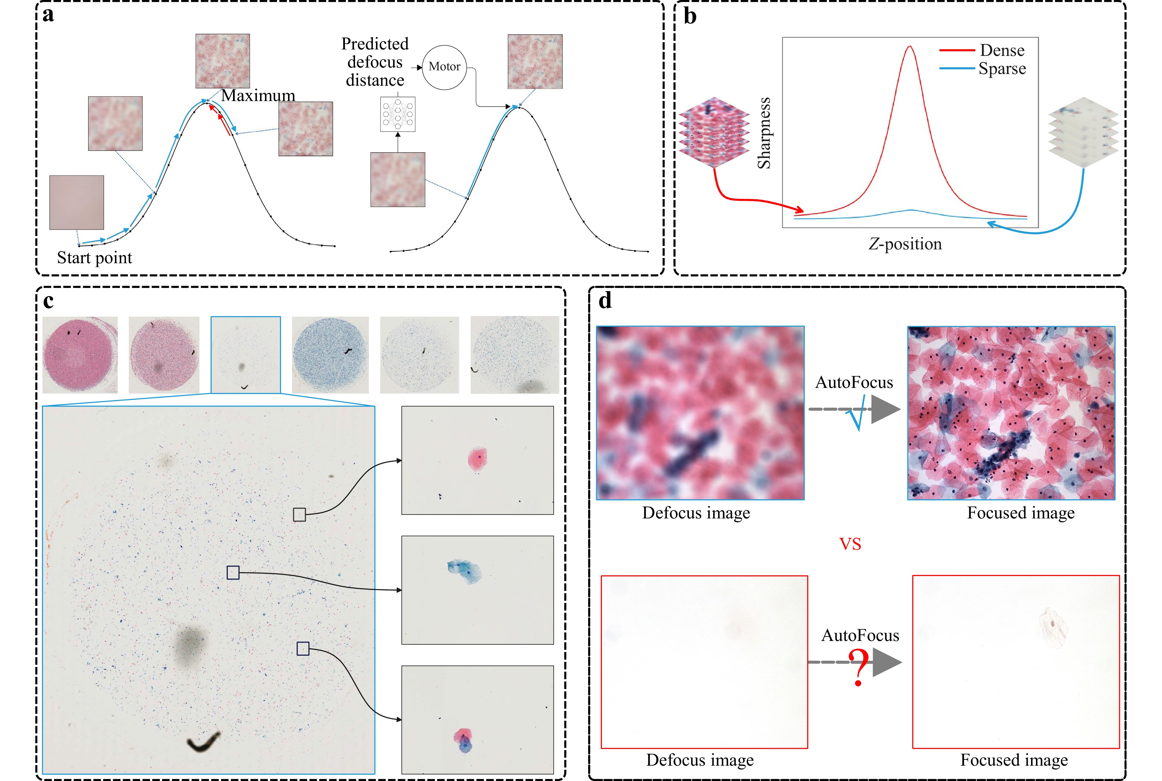
Fig. 1  The sparsity challenge in microscopy autofocus. a One-shot methods employ neural networks to predict defocus distance directly, thus bypassing the iterative adjustments required by traditional hill-climbing techniques. b The sharpness curves for dense and sparse scenarios. It is evident that the sharpness curve exhibits significant variations in dense content, whereas the changes are less pronounced in sparse content. c Images of typical pathological slides, with the upper section showing WSI thumbnails. We display both the cases of dense and sparse content therein. We enlarge one of the sparse samples and randomly select three representative fields of view, each containing only a few cells. d This observation raises a critical question: can autofocus be effectively achieved in sparse-content scenarios?

Over the years, researchers have devised various techniques for autofocus, leading to two dominant methodological streams: active and passive methods. Active autofocus systems¹⁴⁻¹⁹ are characterized by the use of specific optical components to focus on a chosen point or area. For example, the laser triangulation technique is commonly used for autofocus in photolithography^14,15, where the angles in a triangle are measured to determine unknown defocus distances. The Coaxial Defocus Detection method^16,17 leverages the shape and associated parameters of the laser spot to measure the defocus distance. A practical application of this can be seen in the Nikon Perfect Focus System (PFS)¹⁸, which employs near-infrared light to identify a reference plane and subsequently adjust the focus in real time. Phase detection autofocus (PDAF)¹⁹ mainly involves the design of specific CMOS sensors to calculate the focus plane, as exemplified in Nikon DSLR cameras. Despite the rapid speed and high robustness offered by active autofocus systems, their considerable cost, large size, and limited precision present significant limitations in numerous applications.

In contrast, passive autofocus methods²⁰⁻²² achieve focus by analyzing the captured image, regardless of hardware modifications²³. They do not require a specific light path or sensor, nor do they emit probing light. More specifically, passive methods can be further classified into two distinct categories: reference-based and non-reference-based. The most typical example of reference-based methods²⁰ is the hill-climbing algorithm²¹. This method controls the z-axis of the microscope to move up and down to detect contrast changes of the captured image, identifying the high-contrast image that signifies correct focus. Although this method offers high accuracy, its speed is compromised due to the need for multiple mechanical adjustments of the microscope.

Recent advances in microscopy focus on accelerating the autofocus speed to facilitate applications such as dynamic cell tracking²⁴ and WSI scanning¹¹. This has led to the development of non-reference-based (one-shot) autofocus methods that infer the defocus distance directly from a single captured image using regression schemes, primarily employing neural networks²². The pioneering work by Ref. 25 introduced a Convolutional Neural Network (CNN) to predict defocus distance, training a ResNet on approximately 130,000 images with varying defocus distances to establish a mapping between captured images and their corresponding defocused distances. Building on this work, Ref. 22 integrated additional off-axis illumination sources and utilized a Fully Connected Fourier Neural Network (FCFNN) for defocus distance estimation. Meanwhile, Ref. 26 employed the MobileNetV2 network, comparing pixel-wise intensity differences between two defocused images to predict defocus distance. Further innovations include Ref. 27 and Ref. 28, who both utilized the MobileNetV3 network²⁷. achieved defocus estimation without requiring additional light sources, while Ref. 28 incorporated a programmable LED array as the illumination source. Recently, Ref. 29 introduced a two-step process, involving a defocus classification network to determine the direction of defocus and a subsequent refocusing network to estimate the defocus distance. Lastly, Ref. 30 proposed the Kernel Distillation Autofocus (KDAF) method, leveraging virtual refocusing to estimate defocus distance.

In this paper, we highlight a significant challenge that has hardly been noticed in previous methods. This challenge emerges from our observation that in real-world microscopic imaging, the captured content is often sparse. This leads to a majority context of the image being blank, offering no assistance in estimating the defocus distance. Although previous methods employ a patch-based strategy, inferring the focal distance by sampling the observation image into patches and using a voting scheme to achieve a result, our experiments indicate a substantial decline in performance when this situation arises.

To address this, we propose a content-importance-based defocus distance estimation method, named SparseFocus, which is capable of handling autofocus issues across all levels of content sparsity, whether dense, sparse, or extremely sparse. This approach overcomes the limitations of current passive focusing methods in dealing with sparse issues, opening up new possibilities for autofocus in practical applicability. Specifically, we first assign varying importance scores to different regions of the image using a fully convolutional network. Regions with dense content are assigned higher importance scores, regions with sparse content are given lower importance scores, and regions without content are assigned nearly zero importance scores. After that, we select the top-k regions with the highest importance scores and input them into the defocus distance regression network. Based on the defocus distance for each region, we apply a pooling operation to derive the final result.

To train and infer our algorithm, we develop an automated microscopic imaging platform to automatically gather labeled defocused images from microscopic samples. The observational content of this dataset includes pathological tissues and cells, and it accounts for both sparse and dense scenarios. Extensive experiments on this dataset indicate that our method achieves state-of-the-art performance, surpassing previous methods by a significant margin, especially in sparse instances. Notably, even in extremely sparse scenarios, where only one region contains useful content, our method yields satisfactory results.

Data Capturing Considering the scarcity of large-scale, labeled dataset suitable for our network training, we have developed an automated system for microscopic image acquisition coupled with an auto-labeling framework. Please refer to Section 4 for more information about our automated microscopy system.

To improve the sample diversity, we obtain a large collection of pathological tissues and cellular specimens, including samples from the lung, liver, prostate, and exfoliated cervical cells. The cells are stained using Papanicolaou stain, while the tissues are stained with Hematoxylin and Eosin (H&E). Specifically, we first collect 400 samples from patients of different ages and diseases, and then retain 75 cell samples and 63 pathological tissue samples, considering the distinct similarity of most samples. After that, we categorize the data collection into 6 distinct groups according to the type (cell or tissue) and sparsity (dense, sparse or extremely sparse) of the data. Selected samples are illustrated in the supplementary material. For each sample, we randomly selected at least 90 fields of view, each with a resolution of 2016 × 2016 pixels. To collect defocus data, a sequence of z-stack images was captured at 101 different defocus distances, with a step size of 0.5 µm ranging from −25 µm to +25 µm. In total, we obtain 1,344,411 pathological microscopic images with image-level defocus distance labels.

Content Importance Labeling Beyond image-level defocus distance labeling, we introduce patch-level importance assignment for each image. To achieve this, we employ an automated approach exploiting sharpness variations between defocused images and their in-focus counterparts captured within the same field of view. This methodology quantifies the relative contribution of individual regions on defocus prediction. Further methodological details are provided in the supplementary materials.

Statistics We categorize the data based on sparsity and type into six groups. For cells, we have 3345 dense, 2054 sparse and 1824 extremely sparse z-stacks. For tissues, we have 2923 dense, 1442 sparse and 1723 extremely sparse z-stacks. These are then divided into training, validation, and test sets in an 8:1:1 ratio, ensuring a comprehensive and balanced evaluation of our method.

In learning-based autofocusing methods, Mean Absolute Error (MAE) of the predicted defocus distance is often employed to evaluate their performance. However, relying solely on the MAE for assessment has some limitations. For example, it does not indicate whether the estimated defocus distance falls within the Depth of Field (DoF), nor does it reveal if the defocus direction is incorrectly estimated. As a result, we introduce two additional metrics: DoF-Accuracy (DoF-Acc) and Direction Success Score (DSS). The DoF-Acc evaluates the degree to which the predicted focus point falls within the DoF, providing a comprehensive measure of how well an algorithm can achieve autofocus, especially for microsystems with varying parameters and distinct DoFs. The DSS quantifies the precision of the direction prediction. We introduce this metric because an incorrect direction prediction by the autofocus algorithm can lead to more severe image defocus, potentially placing the defocus distance outside the system’s operational range and preventing successful focus resolution.

The MAE quantifies the accuracy of the autofocus algorithm by determining the average absolute difference between the predicted and true defocus distances, which is calculated as:

where $ e_{d_i} $ represents the absolute error, $ \hat{d_i} $ is the predicted defocus distance, $ d^*_i $ is the ground truth defocus distance, and $ |D| $ is the number of samples in the test dataset.

DoF-Acc measures the percentage of absolute errors $ e_{d_i} $ that fall within $ 1/n $ DoF (in this study, we set $ n \in \{1, 2, 3\} $), allowing for a fair comparison between optical microscope systems with different DoF. DoF-Acc is defined as:

The indicator function $ \mathbb{I}(P) $ is defined as:

The DSS measures the percentage of cases where the predicted direction of defocus aligns with the true direction, which is defined as:

where $ \operatorname{sgn}(x) $ is the sign function, defined as:

For the “boundary” case where $ d^*_i = 0 $, indicating that the image is already in focus, the predicted defocus direction, whether positive or negative, can be considered correct.

We conduct an extensive evaluation of our algorithm's performance utilizing the large-scale dataset that we have assembled. To demonstrate the performance of our method, we compared it with several learning-based baselines, including those proposed by Dastidar et al.²⁶, Liao et al.²⁷, Jiang et al.²⁵ and Li et al.²⁹. For each baseline, we partition the image into non-overlapping patches in grid mode, infer the defocusing distance of each patch, and get the result by a median filter operation. To maintain the fairness of the experiments, all baseline models are trained under the same condition as our proposed method, including the use of the same dataset and hyperparameter settings (such as learning rate, batch size, and number of iterations).

First, we evaluated our method using randomly selected samples from each z-stack, as presented in regression plots in Fig. 2a-i, which presents the testing results, encompassing scenarios of high density, sparsity and extreme sparsity. The test results demonstrate that our method significantly outperforms the baseline, particularly under sparse and extremely sparse conditions. The majority of our method's predictions fall within the DoF, unlike comparing baselines, which exhibit substantial incorrectness and frequent directional errors, rendering them incapable of accurate focusing under such conditions. More comparative experiments with other baselines are provided in the supplementary materials.

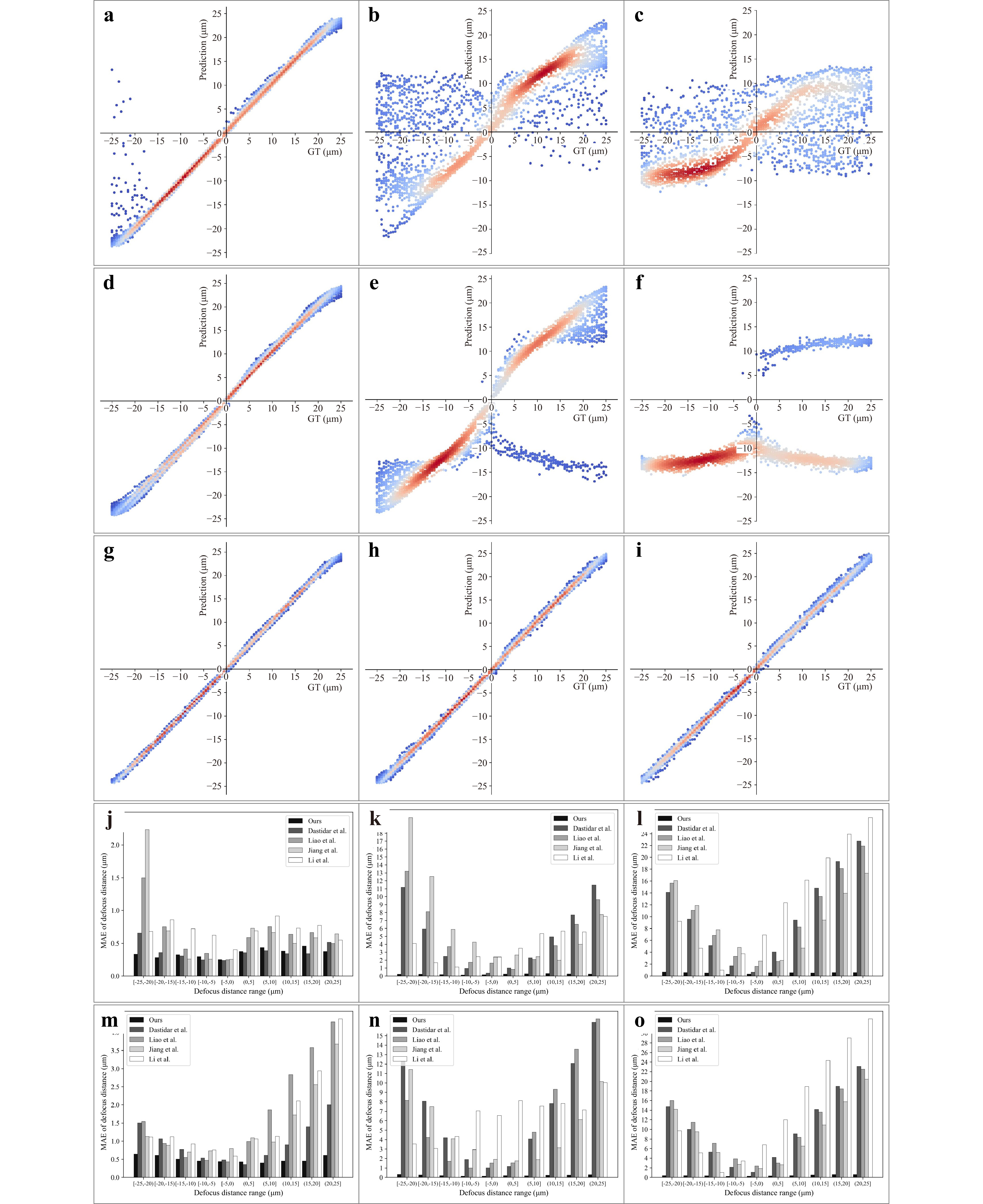
Fig. 2  Performance comparison is conducted via regression plots and error bar charts across different defocus intervals. a-c The regression plots for Jiang et al.’s method²⁵ under dense, sparse, extremely sparse conditions, with the x-axis representing defocus distance (ground truth) and the y-axis showing predicted values. d-f The regression plots for Li et al.’s method²⁹ under dense, sparse, extremely sparse conditions. g-i The regression plots for our method under dense, sparse, extremely sparse conditions. j-l The error bar charts comparing our method and baseline methods on cell samples under dense, sparse, extremely sparse conditions across different defocus intervals, with the x-axis representing defocus distance range and the y-axis showing MAE. m-n The error bar charts comparing our method and baseline methods on tissue samples under dense, sparse, extremely sparse conditions across different defocus intervals.

To further evaluate our method's performance across varying defocus distances, we divided the defocus distance into non-overlapping intervals and calculated the MAE for each interval. As shown in Fig. 2j-o, it can be observed that while the MAE of almost all methods increases with greater defocus distance, the degree of increase varies significantly. In dense scenarios, the MAE remains relatively stable across defocus distances. However, in sparse and extremely sparse scenarios, baseline methods exhibit a significant rise in MAE as defocus distance increases. For example, in sparse tissue samples, the MAE of Dastidar et al.²⁶ increases from approximately 1 µm to about 16 µm, resulting in autofocus failure. In contrast, our method shows minimal sensitivity to varying defocus distance, consistently maintaining low error levels regardless of the initialization to the focal plane.

Next, we assess the performance of the proposed method using the three metrics defined in this paper: MAE, DoF-Acc and DSS. Table 1 presents a comparative analysis of the MAE for predicted defocus distances. The results demonstrate that our method consistently achieves the lowest MAE and standard deviation across all conditions, regardless of the sparsity of the data content. Notably, for images with sparse content, our method surpasses previous methods by a very large margin, reducing the MAE by an order of magnitude. This improvement is particularly striking when considering images with extreme sparsity, where our method successfully performs autofocus with remarkable accuracies of 0.60 µm for cells and 0.45 µm for tissues, while other baselines basically fail. This finding highlights the accuracy, stability, and robustness of the proposed method.

The effectiveness of our method is also substantiated through the DoF-Acc, as illustrated in Table 2. While achieving comparable performance in dense scenarios, our method exhibits a significant advantage in sparse and extremely sparse cases. In sparse situations, the defocus distances predicted by other baselines often fall outside the DoF, leading to unsuccessful autofocus. In contrast, our method consistently achieves accurate focus. For instance, in the extremely sparse case, 58.23% of cell dataset and 71.71% of tissue dataset fell within the DoF.

Table 3 illustrates the DSS. Our method achieves exceptional performance, exceeding 99% for all conditions. In contrast, other methods exhibit numerous incorrect predictions, particularly in sparse and extremely sparse scenarios.

To further verify the critical role of RIN in our method, we conducted ablation experiments comparing SparseFocus with a variant excluding RIN. Specifically, the RIN-removed variant directly feeds all patches into the DPN and applies median filtering to the patch-level predictions to generate the final result. To visually demonstrate the impact of RIN, we plotted MAE versus sparsity curves for both approaches and included visualizations on dense, sparse, and ex-sparse samples, as displayed in Fig. 3. These results show that as sparsity increases, the MAE of the method without RIN rises significantly. In contrast, SparseFocus method consistently maintains substantially lower MAE levels across all sparsity conditions, robustly confirming the essential function of RIN.

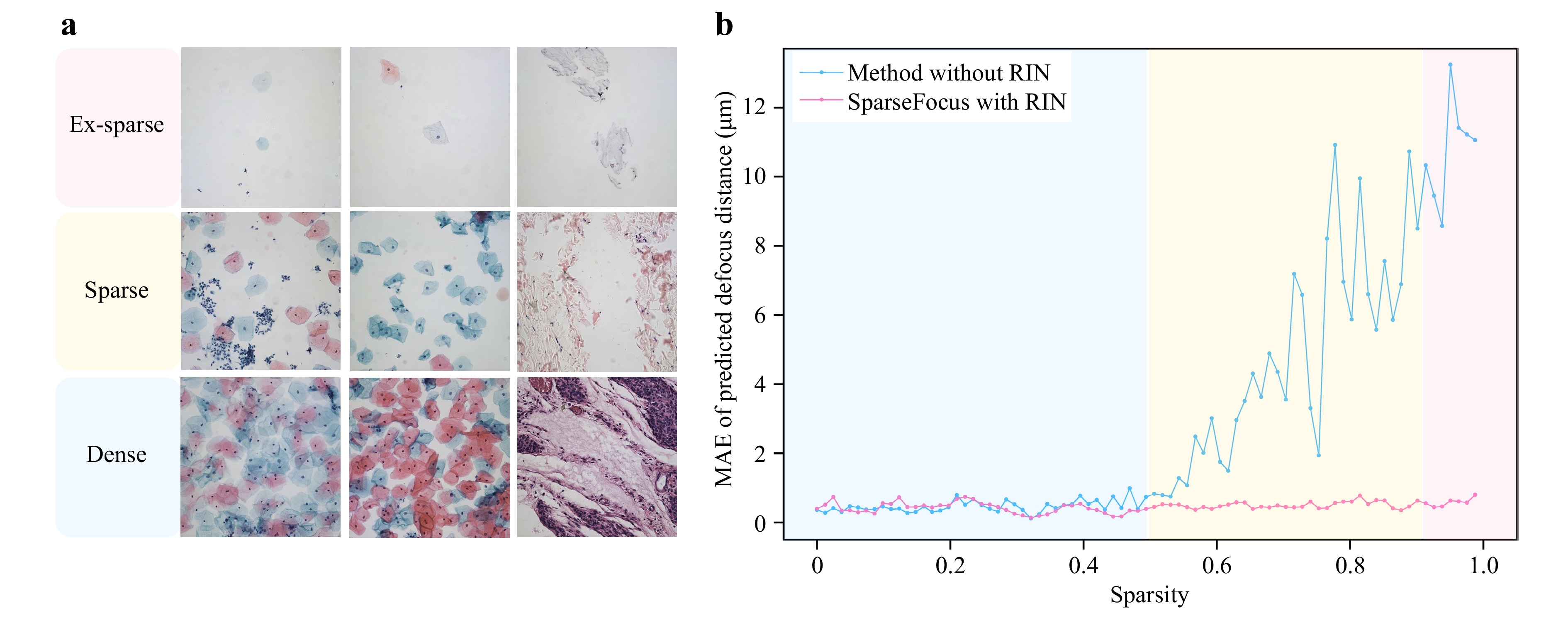
Fig. 3  Comparisons between the SparseFocus method and its RIN-removed variant highlight the essential role of RIN in maintaining low MAE under increasing sparsity. a Typical image samples illustrating different sparsity. b Line plots of MAE versus sparsity for SparseFocus with and without RIN.

Additionally, we conducted ablation and lightweighting experiments by reducing the depth of feature extraction layers in DPN, resulting in performance degradation across all evaluation metrics. Especially in sparse and extremely sparse scenarios, both the MAE and standard deviation of defocus predictions increased significantly. This increase was primarily due to a small number of outliers with large prediction errors, while the majority of the results still conformed to the expected distribution. Comprehensive experimental evidence supporting this observation is provided in the supplementary material.

Meanwhile, we compared our method against traditional hill-climbing algorithms. Given the high parametric freedom in hill-climbing search strategies (e.g., coarse/fine step sizes, stopping criteria), we exclusively employed MAE to evaluate focusing accuracy, as alternative metrics lack reliability under variable configurations. Our method demonstrates superior performance to hill-climbing autofocus in both MAE and computational efficiency. Extended comparative analyses are provided in supplementary material.

In the ideal imaging model, the Point Spread Function (PSF) of a microscope is symmetric with respect to the focal plane. This symmetry allows algorithms to estimate the absolute defocus distance but prevents them from determining whether the defocus is above or below the focal plane, thereby rendering one-shot autofocusing seemingly impractical. However, in real optical microscopy systems, the PSF often exhibits significant asymmetry due to refractive index mismatches among the different media in the imaging path, such as the slide, sample, cover slip, and the surrounding medium like air or immersion oil. These mismatches introduce aberrations, including spherical aberration, coma, astigmatism, field curvature, and distortion, which disrupt the ideal symmetric distribution of the PSF. Fig. 4a, b illustrate the differences in pixel grayscale values at the same position for images at 5 µm and −5 µm. Fig. 4c, d show images at symmetric defocus distances on both sides of the focal plane. Fig. 4e, f present the 3D PSF and 2D PSF of our developed WSI device. These visualizations are generated using the Gibson & Lanni PSF model³¹ within the open-source software Fiji³² and the PSF Generator plugin³³. These visualizations also demonstrate that, in real optical microscopy systems, the PSF is asymmetric. Additional theoretical analysis on the PSF is provided in the supplementary materials.

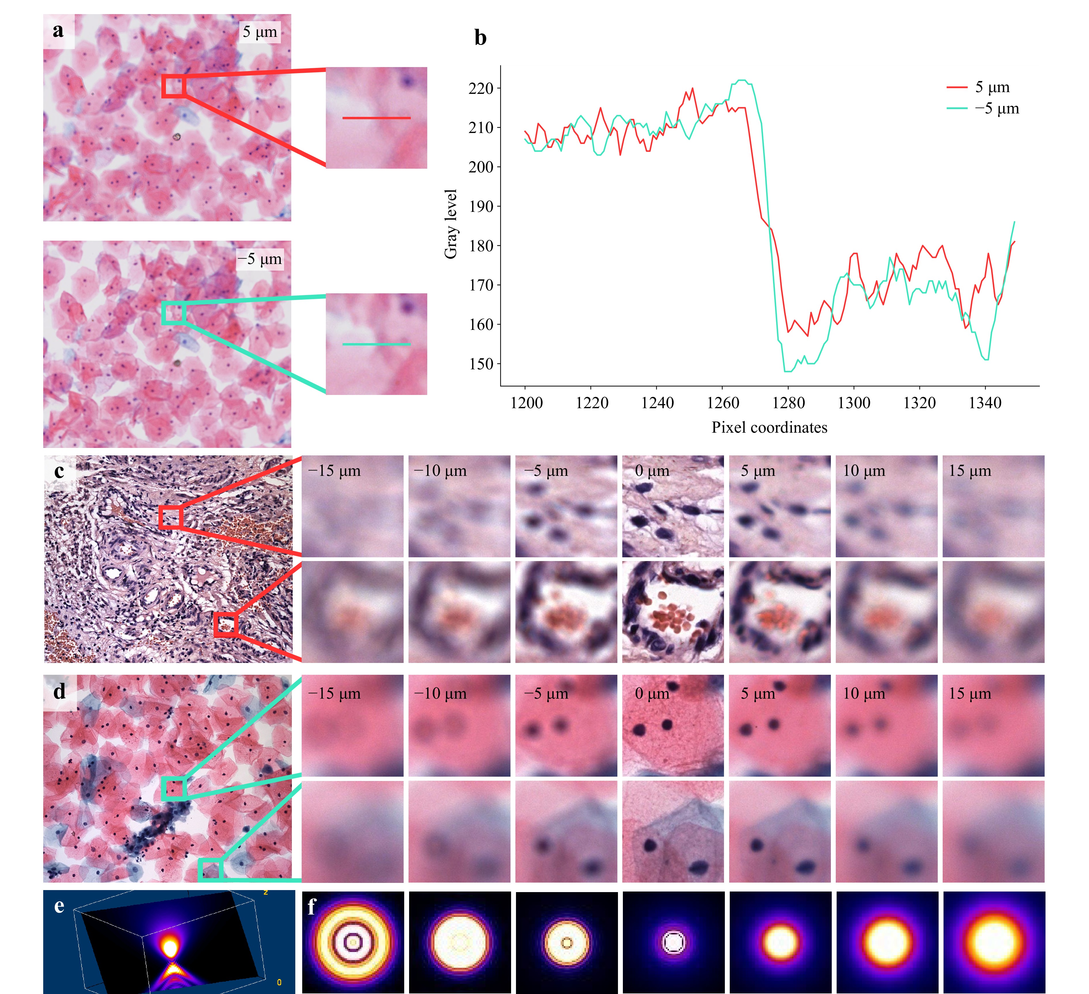
Fig. 4  The asymmetry of PSF. a The images and enlarged details of a specific cell sample at defocus positions of 5 µm and −5 µm. b The gray level variation along the pixel coordinates at the positions indicated by the red and cyan horizontal lines in a. Both of them provide corroborative evidence for the disparities in images at the corresponding locations. c-d The contrast in a specific tissue/cell sample with positive/negative defocus.e The display of the PSF in 3D space. f PSF variations across multiple z-positions in the x-y plane, highlighting its asymmetry with respect to the focal plane.

The asymmetry of the PSF, though potentially detrimental to image quality, presents a unique opportunity for one-shot autofocusing. This phenomenon results in images with positive or negative defocus on either side of the focal plane exhibiting distinct characteristics. Although these differences are subtle, the sophisticated feature extraction capabilities of deep learning can effectively discern them. By capitalizing on this physical principle, we propose a one-shot learning-based network designed to estimate both the defocus distance and direction from a single image.

Autofocus is generally designed for a specific focal plane, assuming that most samples exhibit little variation in elevation over a field of view. However, for very thick samples, such as those resulting from the slicing of pathological sections, different regions within the same field of view may lie on different focal planes (see supplementary material). This can lead to a scenario where focusing on one region causes others to appear blurry, complicating autofocus efforts. To address such challenges, strategies may contain: 1) Designate a specific region of interest for the autofocus algorithm to target exclusively; 2) Employ z-stack image fusion strategy, capturing and fusing images at various z-axis positions to achieve a uniformly sharp image across the entire field of view.

We propose a learning-based two-stage network incorporating Region Importance Network and Defocus Prediction Network to enable autofocus for both dense, sparse or even extremely sparse microscopy images under the one-shot setting. Our method can effectively identify local regions with important content and subsequently estimate the defocus distance using these regions. We also introduce a new large-scale dataset that provides a variety of defocused images with dense and sparse scenarios. Experimental results demonstrate that our method significantly improves defocus distance estimation accuracy compared to existing learning-based one-shot methods, especially in sparse scenarios. Building on this method, we develop a WSI system that exhibits promising focusing capabilities in real-world applications.

An overview of our method is shown in Fig. 5a. Given a defocused image $ \mathbf{I} $ as input, our objective is to calculate the defocus distance $ \hat{d} $ for it. To achieve this goal, we propose a novel two-stage pipeline. In the first stage, the captured defocused image is fed into a fully convolutional network termed Region Importance Network (RIN) $ \mathcal{F}_w $, which simultaneously predicts the important weights $ \hat{\mathbf{W}} = \{ \hat{W}_1, \hat{W}_2,..., \hat{W}_n \} $ for all uniformly-split patches $ \mathbf{P} = \{ P_1, P_2,..., P_n \} $ in the image. In the second stage, Top-k patches $ \mathbf{P}_k = \{ P_i \} $ with the highest weights are selected, and a neural network named Defocus Prediction Network (DPN) $ \mathcal{F}_d $ is used to predict the defocus distance $ \{ \hat{d}_i = \mathcal{F}_d(P_i) \} $ for each patch. Finally, an aggregate operation, i.e., median filtering, is used to obtain the final result $ \hat{d} $. This estimated result $ \hat{d} $ drives the control system, precisely positioning the objective lens at the focus plane for optimal image sharpness.

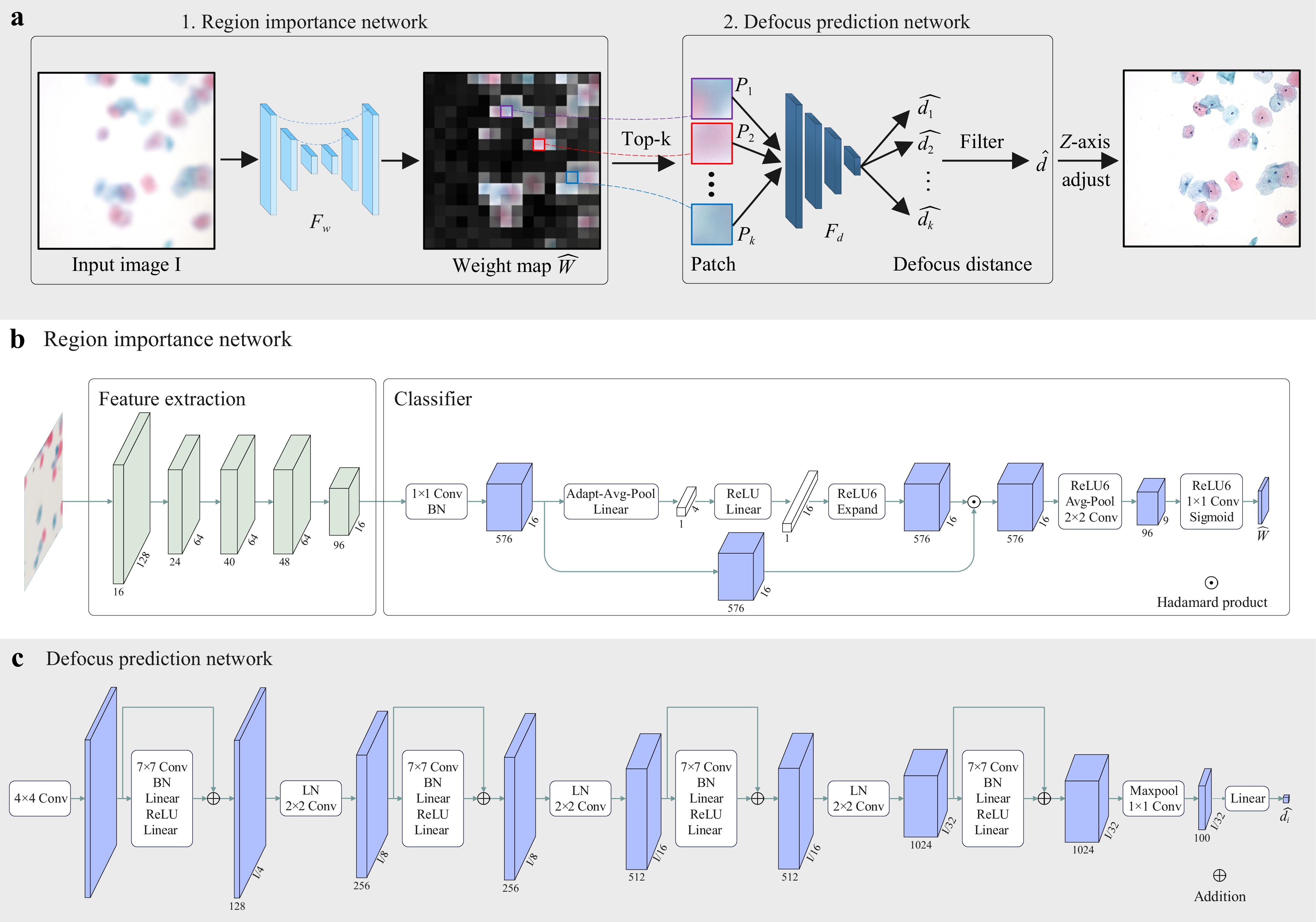
Fig. 5  Framework of the SparseFocus Network. a The overview of our method (SparseFocus). A defocused image is processed by the RIN to compute patch-wise importance weights $ \hat{\mathbf{W}} $, then top-k weighted patches undergo defocus distance prediction via the DPN, followed by median-based aggregation to output the final distance $ \hat{d} $, which guides lens positioning for optimal focusing. b The structure of the RIN, built upon MobileNetV3. The network processes a downsampled 512 × 512 defocused image to generate a 9 × 9 importance score matrix $ \hat{\mathbf{W}} $. Top-$ k $ patches are selected from the original-resolution image using $ k_d $/$ k_s $/$ k_{es} $ thresholds according to dense/sparse/ex-sparse scenarios. c The structures of the DPN. This architecture initiates with a 4 × 4 strided convolution layer coupled with BatchNorm2d to extract hierarchical features and strategically utilizes DFE blocks with 7 × 7 large-kernel convolutions, explicitly designed to capture long-range spatial dependencies distinct from traditional 3 × 3 operators. Sequential downsampling and max pooling stages refine multi-scale representations, enabling regression-based predictions for pixel-aligned defocus distances $ \{\hat{d}_1,...,\hat{d}_k\} $. Finally, a median filtering operation stabilizes the outputs, generating the robust final estimation $ \hat{d} $.

We construct the RIN (shown in Fig. 5b) $ \mathcal{F}_w $ based on MobileNetV3³⁴, which is tailored to assign importance scores to image patches $ \mathbf{P} = \{ P_1, P_2,..., P_n \} $ within a defocused input $ \mathbf{I} $. Specifically, the process begins with cropping the original 2448 × 2048 pixel image $ \mathbf{I} $ to a 2016 × 2016 square, followed by resizing to 512 × 512 pixels. This preprocessed image is then fed into RIN, which outputs a 9 × 9 prediction matrix $ \hat{\mathbf{W}} = \{ \hat{W}_1, \hat{W}_2,..., \hat{W}_n \} $. Each element $ \hat{W}_i $ in $ \hat{\mathbf{W}} $ quantifies the content importance of the corresponding 224 × 224 pixel patch $ P_i $ within the original image $ \mathbf{I} $. We rank all patches $ \mathbf{P} $ based on important scores and select the top-$ k $ most important patches $ \{P_1, P_2,..., P_k\} $ for subsequent processing. The value of $ k $ is denoted as $ k_d $ for dense, $ k_s $ for sparse and $ k_{es} $ for extremely sparse scenarios.

We introduce the DPN (shown in Fig. 5c) $ \mathcal{F}_d $ to predict defocus distance for each selected patch ($ \{ P_1, P_2,..., P_k \} $). Initially, input patches are processed by a 4 × 4 convolution with stride 4 and BatchNorm2d. These features are then refined through multiple Defocus Feature Extraction (DFE) blocks and downsampling modules. In contrast to prior networks that rely on 3 × 3 convolutions, the DFE block utilizes large kernel convolutions (7 × 7), enabling the model to capture comprehensive spatial information and long-range dependencies within the input patches. Furthermore, a max pooling layer is incorporated to retain the most salient features before they are fed into a linear regression layer for defocus distance prediction $ \{\hat{d}_1, \hat{d}_2,..., \hat{d}_k\} $. At last, a median filtering is employed to return the final result $ \hat{d} $.

The overall loss function $ \mathcal{L} $ comprises two components: the RIN loss $ \mathcal{L}_w $ and the DPN loss $ \mathcal{L}_d $.

Importance Prediction Supervision The loss function for the $ \mathcal{L}_w $ is the Binary Cross-Entropy (BCE) Loss³⁵, calculated between the prediction matrix $ \hat{\mathbf{W}} $ and the Content Importance matrix $ \mathbf{W}^* $. Let $ N $ denotes the total number of elements in $ \hat{\mathbf{W}} $ or $ \mathbf{W}^* $, and let $ i $ and $ j $ denote the indices along the $ x $ and $ y $ axes, respectively, the loss function for $ \mathcal{L}_w $ is given by:

Defocus Prediction Supervision The loss function for $ \mathcal{L}_d $ is the $ \mathcal {L}_2 $ loss. For each selected patch $ P_i \in \{ P_1, P_2,..., P_k \} $, we obtain the true defocus distances $ d^*_i \in \{ d^*_1, d^*_2,..., d^*_k \} $. The loss function for $ \mathcal{L}_d $ is:

where $ M $ is the number of patches labeled as positive in the predicted matrix $ \hat{\mathbf{W}} $. $ D = {\hat{d}_1, \hat{d}_2, \ldots, \hat{d}_k} $ represents the predicted values from the DPN.

During training, we augmented the data diversity by adjusting image brightness, contrast, and saturation. Brightness was varied within the range [0.9, 1.4], while contrast and saturation were adjusted within [0.8, 1.5]. Our model was trained for 600 epochs on four NVIDIA RTX 3090 GPUs. We used the Adam optimizer with an initial learning rate of 5 × 10⁻⁵ and a batch size of 16 for the RIN. For the DPN, we employed an initial learning rate of 1 × 10⁻⁴ and a batch size of 128.

During inference, only the top-k patches are processed by the DPN. This selective strategy confers dual advantages: eliminating low-importance patches enhances prediction robustness while substantially reducing computational load. Extensive validation confirms $ k = 3 $ suffices for extremely sparse scenes; $ k = 9 $ is optimal for sparse/dense cases. When seeking maximum attainable precision in dense scenarios, $ k $ may be increased to 31, though this yields marginal gains with significant latency penalties. Meanwhile, We impose $ \rho = 0.8 $ as a hard threshold for patch retention, discarding all low-importance patches.

In this section, we introduce an advanced one-shot autofocus-enhanced Whole Slide Imaging system (osa-WSI), based on our learning-based autofocus algorithm, coupled with an efficient image stitching protocol for large-scale imaging and an online motion path planning. The osa-WSI encompasses several key components: Motorized XY and Z Stages offer a resolution of 100 nm in the XY plane and 50 nm in the Z-axis, with repeatability of 400 nm in XY and 150 nm in Z, ensuring precise focusing within the microscope’s depth of field; Macro-Imaging System captures slide thumbnails and identifies specimen regions, using both transmissive and reflective illumination modes; Microscopy Imaging System is designed for high-fidelity imaging of both transparent and opaque samples, equipped with a LED white light source, an APO objective lens, and a global shutter CMOS camera; Motion Control System excels in path planning and camera triggering, enhancing the overall imaging workflow; Integrated Algorithms include autofocus, image stitching, AI-based recognition, and image quality assessment. These technologies establish our WSI system as a cutting-edge tool in the field of pathology. The physical implementation of osa-WSI is shown in Fig. 6.

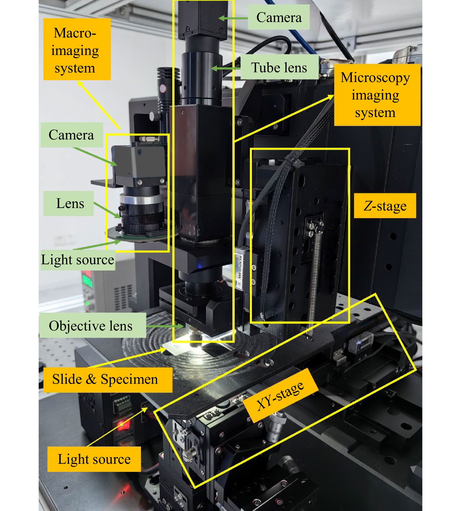
Fig. 6  The real instrumentation of our osa-WSI system comprising its components, which integrates a deep learning-driven autofocus mechanism, a scalable image stitching pipeline, and real-time motion trajectory optimization. The system comprises core modules: motorized stages with high resolution and repeatability; macro-imaging unit; microscopy module with LED white light source, APO objective lens and global shutter CMOS camera; motion control system and AI-based algorithms.

Fig. 7 presents a comparison of the workflow pipelines between the proposed osa-WSI and a traditional WSI system. The traditional system, depicted in Fig. 7a, relies on interpolating from pre-selected Key Focus Points (KFPs) to create a FocusMap for the entire slide, which is inefficient and susceptible to significant errors on uneven sample surfaces. Our osa-WSI system addresses these issues, as outlined in Fig. 7b, c. Fig. 7b describes a two-step process that maintains the FocusMap construction but with improved speed and accuracy. In contrast, Fig. 7c illustrates a one-step process that generates FocusMaps in real-time during scanning, thereby eliminating the need for pre-construction.

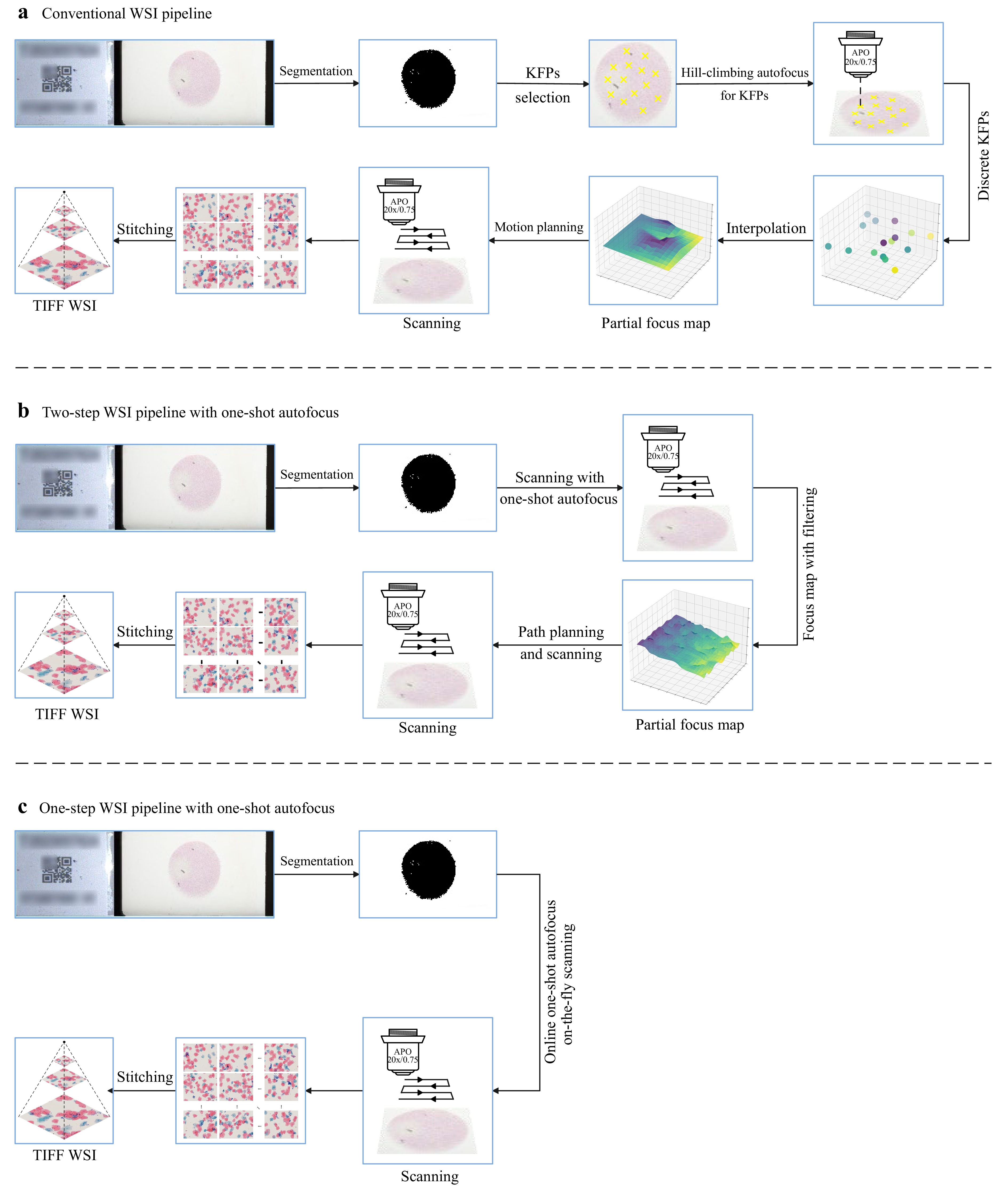
Fig. 7  Overview of three WSI pipelines. a The workflow of a traditional WSI system, which pre-selects KFPs and uses conventional hill-climbing autofocus methods at these positions to create the FocusMap via interpolation, requiring two scanning passes. b The pipeline incorporating one-shot autofocus technology, implemented via a two-step method, which employs our one-shot rapid autofocusing approach to focus all fields of view and create the FocusMap, also requiring two scanning passes. c The dynamic acquisition process of the WSI pipeline using one-shot autofocus, which enables real-time autofocusing during on-the-fly scanning, requiring only a single scan pass.

Fig. 8 shows the FocusMaps and their errors generated by the SparseFocus Model and traditional KFPs interpolation method. Visibly, the SparseFocus method demonstrates superior performance in both cell and tissue samples, as evidenced by its Error Map. This advantage is particularly pronounced in tissue samples exhibiting irregular thickness variations. The traditional method, while guaranteeing focal precision exclusively in pre-selected regions, suffers elsewhere due to the unpredictable thickness changes. These variations lead to substantial deviations between the interpolated results and the actual focal planes in many fields of view. Consequently, large errors manifest within the Error Map, thus introducing significant blurring artifacts into the final WSI result. In contrast, SparseFocus rapidly and accurately predicts the focal plane for each field of view, avoiding the time-consuming operations required by traditional pre-focusing and the higher errors introduced by interpolation.

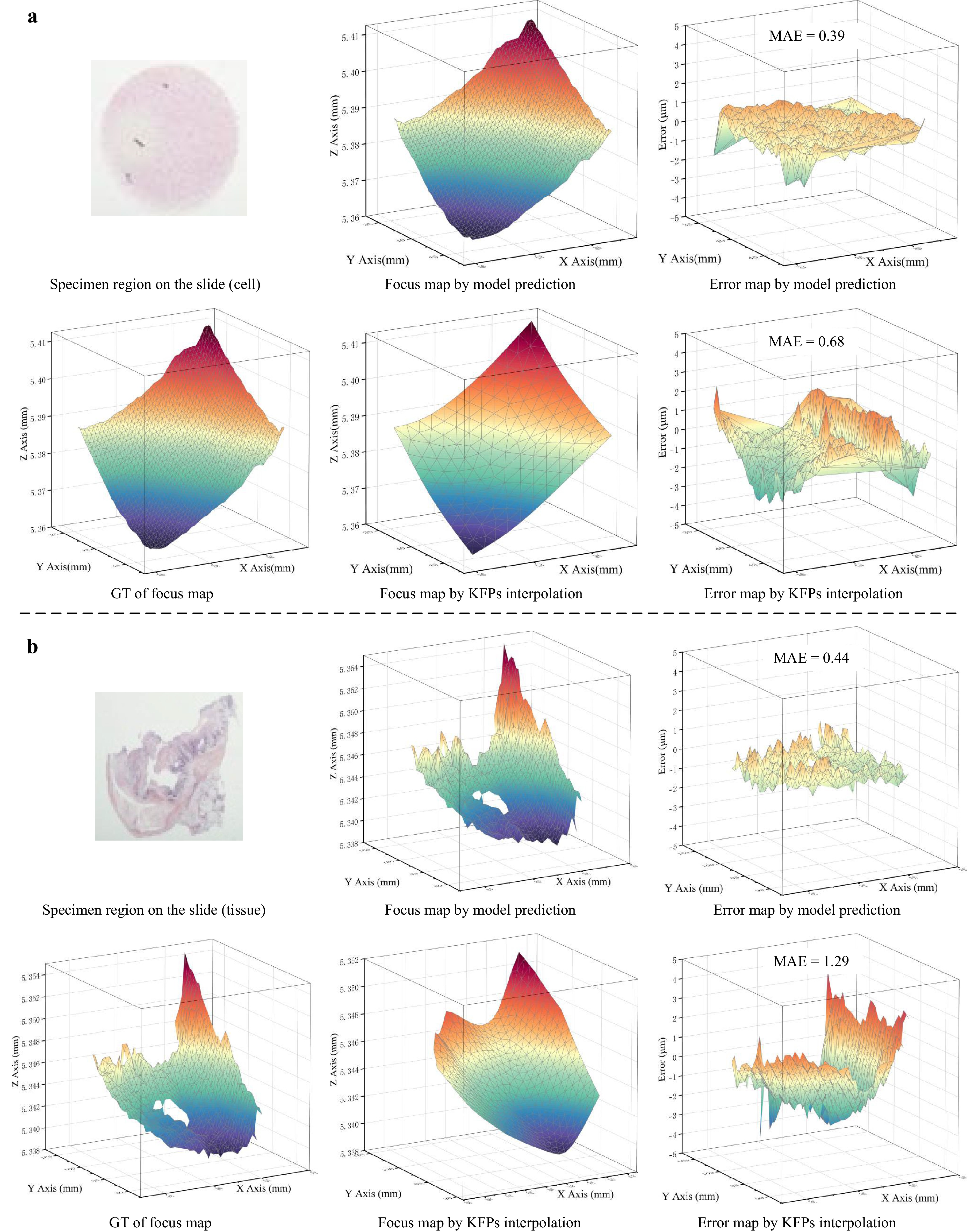
Fig. 8  A comparison between the conventional KFPs interpolation method and SparseFocus Model prediction method by FocusMap and its corresponding error map. a-b We demonstrate: Ground Truth (GT) of FocusMap, FocusMap via KFPs interpolation, FocusMap via Model Prediction, Error Map derived from KFPs interpolation, Error Map derived from Model Prediction both in cell (a) and tissue (b) samples, showing that SparseFocus has significant advantages over the conventional method in practical WSI systems.

This study was supported by the Innovation Research Foundation of National University of Defense Technology (NO.22-ZZCX-064) and the National Natural Science Foundation of China (No. 62406331).