A novel multi-spatial-frequency ultra-precision and efficiency-enhanced manufacturing paradigm based on immersion depth and scanning speed dynamic co-variation model

In extreme ultraviolet lithography (EUVL), the projection objective lens system plays a critical role in achieving high-resolution lithography, with accuracy requirements that reach the sub-nanometer scale¹. In cutting-edge fields such as satellite internet and spaceborne laser communication, the high-precision and high-efficiency fabrication of optics is also essential for enabling the mass construction of high-performance systems^2,3. Aspherical reflectors are key elements in both EUVL projection objective lens systems and optical antennas, where surface accuracy directly impacts imaging performance as well as communication quality or data transmission rates. Besides, the free-form continuous phase plate (CPP) is a vital element for beam smoothing and focal spot shaping in inertial confinement fusion facilities, including the National Ignition Facility⁴ and Shenguang III⁵. Thus, the high-efficiency and high-precision fabrication of complex optics is a fundamental requirement for progress in optical manufacturing.

Existing computer-controlled optical surfacing (CCOS) and its derivative techniques are based on the Preston equation⁶. Magnetorheological finishing (MRF) exhibits high material removal efficiency, low subsurface damage, and excellent surface quality, making it one of the most important optical manufacturing technologies⁷. However, nearly all current paradigms depend on stable TIF and regulate material removal solely through dwell time, which imposes inherent limitations^8–10. Moreover, insufficient control of mid-spatial-frequency (MSF) error remains a critical bottleneck that limits the application of MRF in ultra-precision domains, such as EUVL.

Firstly, the convolution of the constant TIF and dwell time on the regular path primarily introduces MSF error, while simultaneously optimizing low- and mid-spatial-frequency errors within a single pass remains challenging¹¹. Secondly, dwell time limits the dynamic response capability of the system and restricts adaptive optimization of processing parameters¹². Besides, during aspheric element fabrication, the TIF exhibits spatiotemporal instability due to curvature effects, significantly reducing accuracy¹³. In addition, long-term variable acceleration loads on the machine motion system cause error accumulation and degrade stability. Furthermore, extended dwell time (low scanning speed) improves material removal but lowers processing efficiency, whereas shortened dwell time (high scanning speed) reduces removal and compromises surface accuracy. This trade-off between removal efficiency and fabrication accuracy fundamentally limits overall manufacturing performance¹⁴.

The Preston assumption indicates that the material removal amount is determined by both the dwell time and the tool influence function¹⁵. Schinhaerl et al. proposed a polishing method that dynamically adjusts the tool removal capacity via the maximum moving velocity and surface error-profile¹⁶. Su et al. developed a freeform surface generation approach to address the inherently nonlinear and time-variant TIF in atmospheric pressure plasma processing¹⁷. Zhang et al. establish the TIF model based on a modified framework that integrates Archard wear theory and micro-contact mechanics¹⁸. Ji et al. improved stability in atmospheric pressure plasma processing by suppressing the nonlinear fluctuations of the tool influence function¹⁹. Rao et al. proposed a form error compensation in soft wheel polishing by contact, which real-time optimized the time-variant TIF and polishing force²⁰. Sun et al. achieved a time-variant TIF by controlling the belt speed to modulate the volume removal rate²¹. Wan et al. mitigated MSF error in MRF by employing a magic angle-step state, modulating the active region of the TIF²². Although previous studies have demonstrated the substantial impact of time-variant TIF on the material removal, two fundamental limitations remain. First, existing paradigms emphasize passive adaptation of the TIF, addressing thermal effects and tool wear caused by inherent nonlinearities, while lacking any actively controlled dynamic mechanism. Moreover, no quantitative relationship has been established between the time-variant TIF and the deterministic material removal or dwell time solution method. Such limitations prevent current technologies from moving beyond the passive compensation paradigm and fail to satisfy the urgent requirements of precision and efficient optical manufacturing for active control of TIF and efficient and precise convergence of error.

Achieving high-precision and high-efficiency magnetorheological finishing, particularly for suppressing of MSF error, necessitates a comprehensive theory for dynamically optimizing both the profile and removal efficiency of the TIF. Modulating removal efficiency facilitates the flexible regulation of higher scanning speeds, whereas spatial modulation enhances the suppression of MSF error. Furthermore, developing a precise and efficient adaptive compensation strategy for the curvature effect of aspheric surfaces is essential. Establishing a dwell time solution method compatible with shape-variable TIFs and fully leveraging high-speed scanning is also critical for advancing deterministic optical fabrication.

The existing MRF is a deterministic manufacturing technology based on CCOS, as illustrated in Fig. 1. The convolution equation determines the controllable quantitative removal process of CCOS, where the material removal amount Z(x,y) at the surface point (x,y) is the convolution of the tool influence function R(x, y) and the dwell time T(x,y)²³:

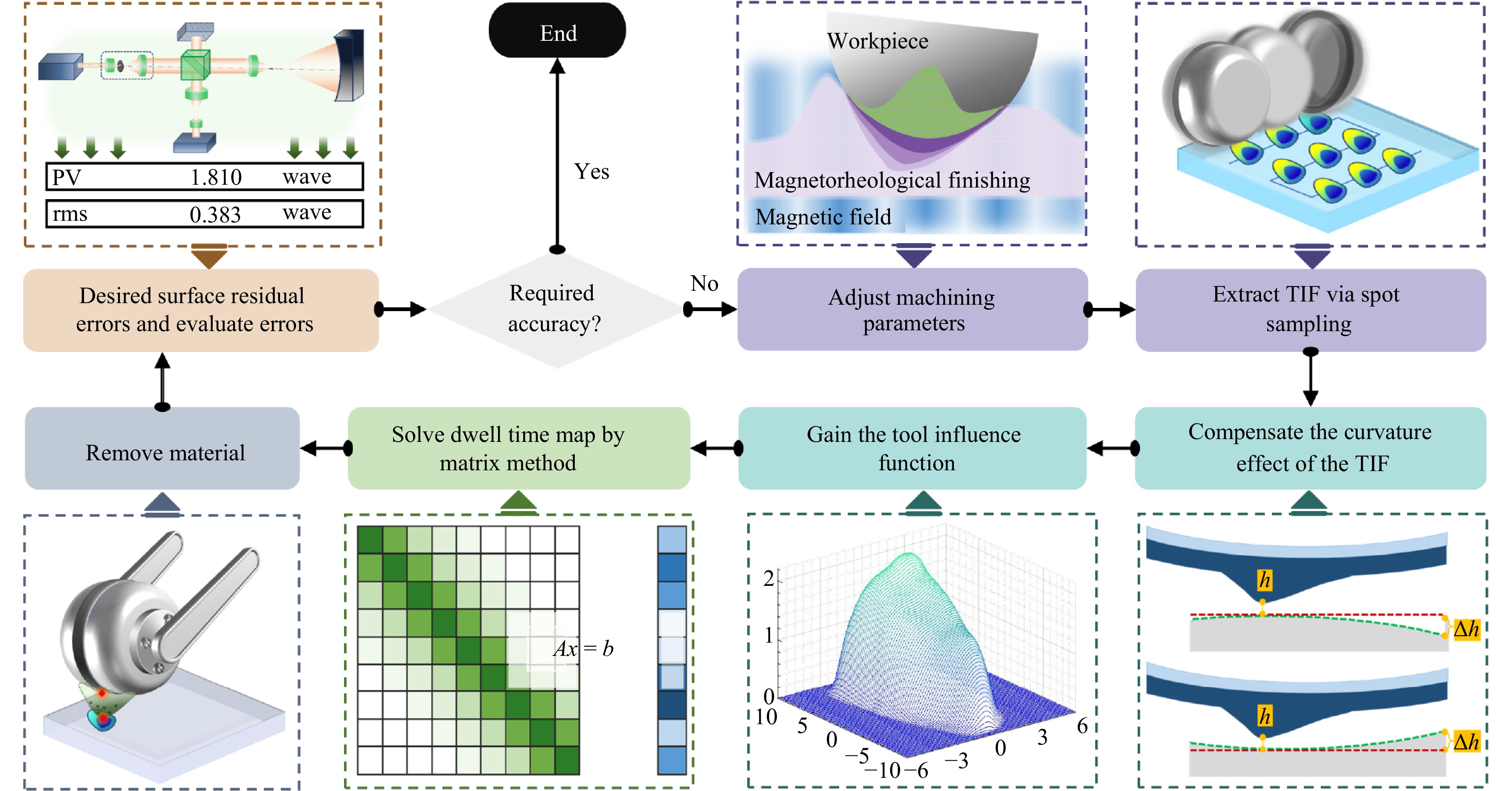
Fig. 1  The process of magnetorheological finishing.

where $ \ast \ast $represents the convolution operation. Therefore, the accurate TIF is the premise of the CCOS.

As shown in Fig.1, spot sampling is a standard method for evaluating the removal capacity²⁴. However, mechanical positioning errors, alignment inaccuracies, and measurement inconsistencies often reduce the accuracy of the derived TIF. During aspheric surface manufacturing, surface curvature variations induce spatiotemporal dynamics in the TIF, violating the assumption of spatially and temporally invariant behavior. Therefore, accurate TIF modeling is crucial for optimizing parameters and achieving deterministic control of time-variant TIF.

Magnetorheological finishing relies on the rheology of magnetorheological (MR) fluid in an external magnetic field. Without the magnetic field, MR fluid exhibits Newtonian behavior. During polishing, the MR fluid circulates through the narrow gap between the workpiece and polishing wheel. Under the strong magnetic field, the magnetic sensitive particles form chain-like structures aligned with the field direction, producing a semi-solid Bingham ribbon^25,26. Bingham fluids exhibit finite yield stress $ {\tau }_{0} $, described by the Bingham equation²⁷.

where τ denotes the shear stress of the MR fluid, η is the plastic viscosity coefficient, and $ \dot{\gamma } $ represents the shear rate. According to Eq. 2, the MR fluid begins to flow only when the shear stress exceeds the yield strength; otherwise, it forms a solid-like core. The following assumptions are made for the MRF region: the MR fluid flow is laminar, and flow in the y-direction is neglected; the MR fluid is incompressible and free boundary effects are ignored; pressure is assumed to be uniform within the layer, and the shear stress is proportional to the velocity gradient.

MRF material removal results from the combined effects of shear stress and dynamic pressure, making accurate evaluation of both components essential for constructing the TIF model. The shear stress and pressure within the polishing region can be analytically described using the lubrication theory of Bingham fluids. As shown in Fig. 2, the gap between the workpiece and the polishing wheel H is divided into several equal segments with the corresponding height h. The distance between the workpiece and the polishing wheel H, immersion depth H_l, and ribbon thickness H_d satisfy the relationship expressed in Eq. 3:

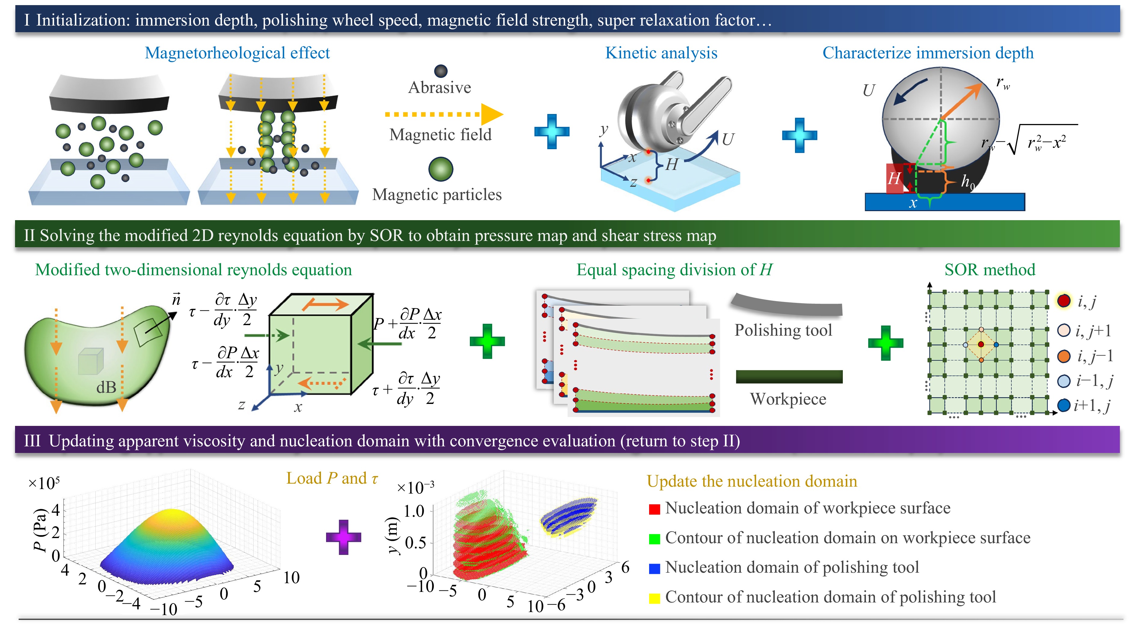
Fig. 2  Calculation flow of pressure, shear stress, and nucleation region in MRF.

Combined with the boundary conditions, the kinetic equation of the polishing area can be expressed by the modified Reynolds equation²⁸:

where $ \overline{\cdot } $ represents dimensionless, P represents the pressure distribution, $ \Lambda $ denotes the aspect ratio of the polishing region, h₀ represents the distance between the lowest point on the polishing wheel and the workpiece, r_w is the radius of the polishing wheel, U is the linear velocity of the surface of the polishing wheel, and µ_i is the unit viscosity coefficient of the MR fluid.

The Reynolds equation is solved following the flow in Fig. 2, employing an over-relaxation iterative method. If the solution fails to meet the predefined convergence criterion, the pressure distribution is updated with over-relaxation and reintroduced into the Reynolds equation for further iteration, yielding converged solutions for both pressure and shear stress. According to τ₀, the solid-state nucleation area within the polishing region is identified, and the apparent viscosity distribution is subsequently updated. The Reynolds equation is solved again with the revised viscosity. Iterative updates continue until the nucleation region converges, yielding steady-state pressure and shear stress distributions.

The material removal efficiency of MRF is significantly influenced by process parameters, the properties of the polishing fluid, and the characteristics of the workpiece material. The process parameters include magnetic field strength, polishing wheel rotational speed, wheel radius, and immersion depth, as illustrated in Fig. 3a. The magnetic field strength determines the stability of the magnetic chain structures, which in turn affects the shear yield stress of the polishing fluid, as expressed in Eq. 5²⁹.

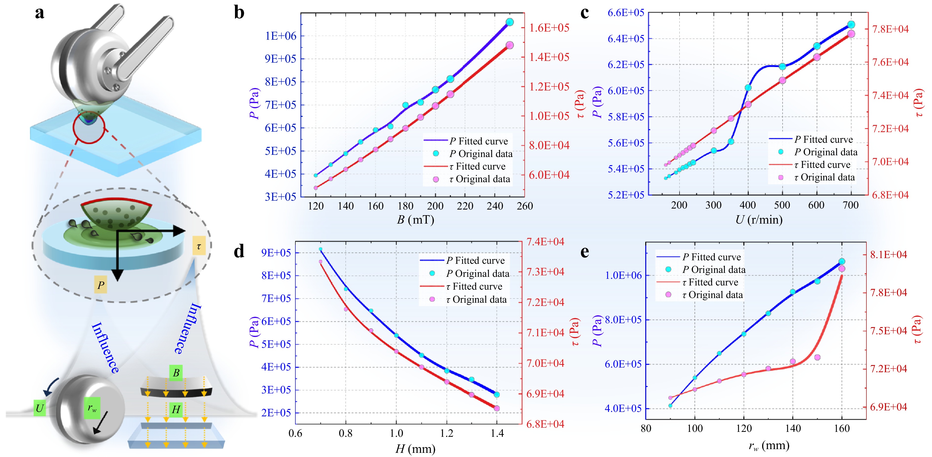
Fig. 3  Shear-dominated removal and shear force under the premise of pressure: parameter influence on pressure and shear stress. a Coupled influence of magnetic field strength, distance between the workpiece and the polishing wheel, wheel rotational speed and radius on the removal efficiency in MRF. b-e Monotonic behavior of B, U, H, r_w with respect to P and τ.

where φ represents the volume fraction of ferromagnetic particles in MR fluid, B is the magnetic induction intensity, r_f and t_f respectively denote the radius and coating thickness of ferromagnetic particles, ρ represents the net distance between adjacent ferromagnetic particles, µ₀ is the vacuum permeability, χ is the magnetic susceptibility of ferromagnetic particles, and ψ represents the shear stress coefficient.

According to Preston's classical removal model, the material removal process can be described in the form of a linear equation³⁰:

Eq. 6 represents a typical power-law model, where MRR denotes the material removal rate at point (x, y) per unit time, and K is the Preston coefficient determined by the manufacturing conditions. Eq. 6 indicates that in sub-aperture polishing technologies, such as CCOS and bonnet polishing, material removal is primarily pressure-driven. However, MRF mainly depends on shear stress, with pressure as a prerequisite for generating shear force. Accordingly, a modified power-law model incorporating both shear force and pressure is proposed.

Magnetic field strength, polishing wheel rotational speed and radius, and immersion depth exert coupled effects on material removal efficiency, it is essential to individually assess whether these parameters exhibit monotonic relationships with shear stress and pressure, which serves as the basis for establishing the modified removal efficiency model that incorporates the interrelations among the TIF, shear stress, and pressure. Control experiments were conducted by varying polishing wheel radius, rotational speed, magnetic field strength, and immersion depth as single-variable factors to solve pressure and shear stress. The fitted curves are shown in Fig. 3. These parameters exhibit monotonic influences on both the magnitude and distribution of pressure and shear stress, supporting the formulation of the modified MRF removal efficiency model in Eq. 7:

By introducing the exponential factor α, the combined influence of shear stress and pressure on MRF removal efficiency is revealed.

The regulation of the polishing fluid by the magnetic field exhibits a saturation threshold. Excessively high wheel rotational speed increases recovery pressure, which may destabilize the circulation system. The flow velocity of the MR fluid is challenging to regulate automatically during processing³¹. In contrast, the immersion depth has a significant influence on the TIF and offers greater adjustability and control accuracy. Hence, the actively controllable spatiotemporally variable TIF driven by immersion depth is proposed. The modulation effect of the TIF is described by Eq. 8:

where $ \Theta ({H}_{l}(x,y,t)) $ represents the modulation effect of immersion depth on the TIF, and $ {R}_{0}(x,y) $ is the reference TIF corresponding to the maximum removal efficiency.

The actively controllable spatiotemporally variable TIFs modulate the removal rate and facilitate effective convergence of low-spatial-frequency error. In regions exhibiting larger surface errors, increased immersion depth enhances material removal efficiency, while reduced immersion depth is applied to areas with smaller errors to avoid overcorrection. Moreover, the ACSV TIF adjusts material removal efficiency and shape contour, thereby suppressing mid-spatial-frequency error.

The Lawrence Livermore National Laboratory defines mid-spatial-frequency error as having a spatial wavelength of 0.12−33 mm³². In the MRF process, the regularly distributed MSF error is significantly affected by the convolution effect of the TIF³³. For the constant TIF, the frequency domain of Eq. 1 is Eq. 9.

where $ \hat{R}({k}_{x},{k}_{y}) $ and $ \hat{T}({k}_{x},{k}_{y}) $ represent the Fourier transform of the constant TIF and dwell time, respectively. During manufacturing, the tool typically performs discrete dwell sampling with a uniform grid spacing Δ. Taking the x-direction as an example, the distribution of the tool influence function R(x) can be modeled as Eq.10:

where R_m represents the TIF value at the position x = mΔ, and $ \delta (\cdot ) $ represents the discrete sampling point. The Fourier transform of Eq.10 is:

The global distribution of the constant TIF is uniform; that is, R_m remains constant. Applying the Poisson summation formula, the Fourier transform of the TIF is given by:

where r₀ represents the density of the reference TIF under the uniform TIF. Substitute into Eq.9, get:

Therefore, the spectrum of material removal includes the product of the TIF spectrum and the periodic pulse sequence. The power spectral density of MSF error can be expressed as:

where W(k) represents the frequency domain window function. According to the MSF error given by the National Key Laboratory of Livermore, the range is k∈[k₁, k₂], k₁ = 0.03 mm⁻¹, k₂ = 8.33 mm⁻¹.

Since $ \hat{Z}(k) $ contains pulses separated by k_s, its squared amplitude is given by:

Hence, in the mid-spatial-frequency range k∈[k₁, k₂], if there exists an integer n such that nk_s∈[k₁, k₂], then the spatial period of the corresponding periodic error component is:

The sampling grid spacing of the polishing path is generally Δ∈[0.15, 1.00] mm, then k_s∈[1.00, 6.67] mm⁻¹. Therefore, there must be k_s∈[k₁, k₂], p_s = Δ, and there may be nk_s∈[k₁, k₂](n ≥ 2). Moreover, the frequency response of the TIF exhibits a low-pass characteristic, with its magnitude attenuating as frequency increases, i.e., $ \left| \hat{R}({k}_{s})\right| $ is generally much larger than $ \left| \hat{R}(n{k}_{s})\right| (n\geqslant 2) $. Thus, the mid-spatial-frequency component with the highest energy corresponds to the fundamental frequency n = 1, leading to a dominant period of the MSF error given by:

Therefore, under the uniform grid, the periodic convolution effect of the constant TIF results in MSF error with the dominant period equal to the sampling interval Δ, as shown in Fig. 4. Let G(x,y) denote the profile of the constant TIF. When the polishing tool is located at point (x,y), the basic expression of the ACSV TIF is defined as:

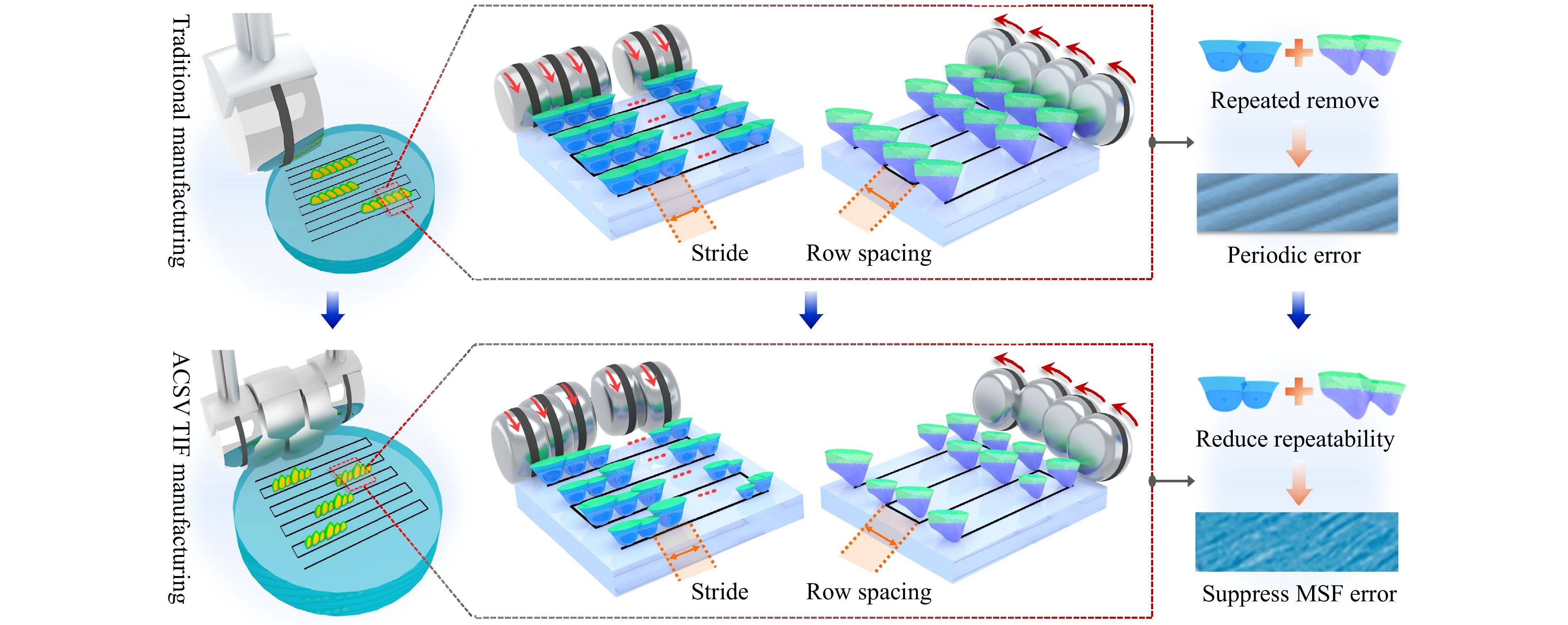
Fig. 4  The generation mechanism of MSF error in the traditional manufacturing paradigm and the ACSV TIF based on variable immersion depth suppresses the MSF error.

where R_var represents the ACSV TIF, R_c represents the reference TIF at the constant immersion depth, υ_e(x,y) represents the material removal efficiency change parameter at (x,y) point, a(x,y) and b(x,y) are the position-dependent shape parameters with the nominal values a₀ and b₀, Δa and Δb denote the variation of shape parameters with spatial position. Limited by the dynamic performance of the machine tool, a(x,y) and b(x,y) vary only slightly within a local neighborhood. Accordingly, the frequency response of the ACSV TIF is:

Due to a and b varying with the randomly changing immersion depth, the global frequency response $ {\hat{R}}_{eff} $ is the expected value of the random frequency response:

where $ \mathbb{E} $ denotes the mathematical expectation. According to probability theory, the expectation of random variables can be expressed as the integral of the original function and its joint probability density function f(a,b):

Based on the theoretical modeling process of the TIF of MRF, the shape parameters a, b, and the removal efficiency parameter υ_e change synergistically and can be parameterized to υ_e = β₁(a), b = β₂(a). Furthermore, the joint probability density function is simplified to a single variable distribution:

Therefore, the frequency response of the ACSV TIF can be regarded as the weighted superposition of the original frequency response and the parameter distribution, which is further simplified into the convolution form. Moreover, since the surface errors of optical elements exhibit random and continuous behavior, the shape parameters a, b, and the efficiency parameter υ_e of the TIF controlling the error are randomly changed and obey the uniform distribution $ a\sim \mathcal{U}[{a}_{0}(1-{\sigma }_{a}),{a}_{0}(1+{\sigma }_{a})] $ with a proportional coefficient of $ {\sigma }_{a} $, whose probability density function is:

Therefore, the frequency response of the ACSV TIF satisfies the relationship:

In summary, the convolution operation expands the discrete δ pulse into a continuous sinc(·) function, dispersing the spectral energy of the original periodic signal into surrounding frequency bands and thereby suppressing energy accumulation at fixed frequency k_s = 1/Δ, as shown in Fig. 4. As a result, the ACSV TIF exhibits a smoothing and suppressing effect on MSF error, effectively enhancing the precision of optical ultra-precision manufacturing.

Temporal and spatial variations in TIF profile and removal efficiency introduce significant complexity into solving dwell time with coordinated requirements for manufacturing precision and efficiency, particularly when employing constant in-row and variable between-row speeds.

For aspheric surfaces, curvature variations introduce spatiotemporal dynamics in the TIF known as the curvature effect. Current compensation strategies commonly approximate the TIFs of local regions on complex surfaces by employing TIFs associated with the closest sphere³⁴, but face apparent limitations: numerous fitting regions increase computational complexity, and fitting errors reduce compensation accuracy and practical effectiveness (Fig. 5). Therefore, accurate compensation for the curvature effect constitutes an essential prerequisite for solving dwell time accurately. The optical surface can be expressed as a polynomial equation, as shown in Eq. 25:

where r_r² = x² + y²; c denotes the vertex curvature; k_o is the eccentricity constant; d₁, d₂, and d₃ represent the quadratic correction coefficients; d₄, d₅, d₆, and d₇ are the cubic correction coefficients. Based on Eq. 25, the first and second derivatives of the aspheric surface in the x- and y-directions are calculated. The first fundamental form coefficients F₁, F₂, and F₃, and the second fundamental form coefficients L₁, L₂, and L₃ are expressed as follows:

Therefore, the Gaussian curvature C_G and the mean curvature C_H are determined respectively：

According to the curvature defined by Eq. 27, the distance between the polishing wheel and the workpiece at each sampling point on the aspheric surface is mapped to the corresponding distance for a sphere of equivalent curvature. Based on the geometric principle, the distance H between the polishing wheel and the sphere is given by Eq. 28:

Concave spherical surface:

Convex spherical surface:

where x represents the coordinates of the polishing area, and r_s represents the curvature radius of the sphere.

The curvature of a spherical surface remains constant at all points. By substituting the distance expression in Eq. 28 into the Reynolds equation, the TIF for the aspheric element mapped onto the spherical surface can be solved, effectively compensating for and eliminating curvature effects (Fig. 5). The pointwise curvature-adaptive compensation method performs separate mapping and theoretical TIF calculation at each point, enhancing compensation accuracy under complex curvature and thereby improving aspheric fabrication precision.

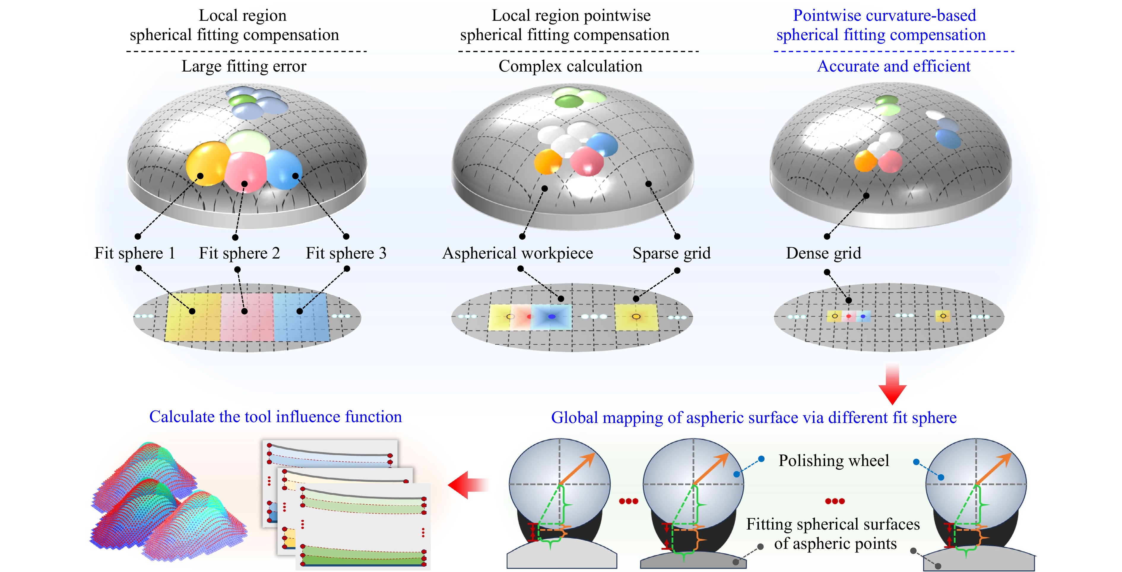
Fig. 5  Comparison and steps of aspheric curvature effect compensation methods.

The influence of immersion depth on the removal efficiency and the shape contour endows the ACSV TIF with error correction capability. To address the limitations inherent in the traditional paradigm, an additional degree of freedom linked to the TIF is incorporated, allowing for increased scanning speed while reducing dwell-time mutations and preventing excessive material removal. However, the TIF at each sampling point exhibits unique spatial characteristics, raising the complexity of dwell time computation. The linear matrix equation method is adopted to solve dwell time³⁵, as follows:

where $ {\boldsymbol{1}}_{\{\cdot \}} $ is the indicator function, which equals 1 when the condition is satisfied and 0 otherwise.  Numx and Numy represent the row and column dimensions of the surface error matrix, and the size of the removal rate matrix is Numm＝Numx×Numy. i represents the current TIF dwell position, j represents the target sampling point, $ (\Delta x,\Delta y) $ represents the relative position of the target sampling point and the dwell point, (O_x,O_y) represents the corresponding TIF center at each target sampling point, and (Tif_x,Tif_y) represents the TIF index value at each dwell point. k_gr and k_gc represent the multiple relationships between the TIF grid and the surface error grid in the row and column directions. nrow_Tif and ncol_Tif define the TIF matrix size at the dwell location. The dwell time is expanded as a vector $ \boldsymbol{t}={[{{t}_{1}},{{t}_{2}},\ldots ,{{t}_{Numm}}]}^{\mathrm{T }} $ according to the column priority, and the surface error matrix E(x,y) is similarly vectorized in column-major order to vector $ \mathbf{e}={[{{e}_{1}},{{e}_{2}},\ldots ,{{e}_{Numm}}]}^{\mathrm{T }} $. The TIFs at all sampling points collectively constitute the removal efficiency matrix M(x,y). The convolution is thereby reformulated as a matrix multiplication, yielding the revised form of Eq. 1 as:

The linear equation is constrained to enforce equal dwell times for adjacent columns within each row, ensuring constant in-row and variable between-row speeds. The corresponding constraint condition is given by:

where T_p,q is the value of the p-th row and q-th column in the dwell time matrix T(x,y). Given that the surface error and the dwell time are both represented as one-dimensional vectors in column-major order, so:

Each constraint T_p,q = T_{p,q + 1} corresponds to a row of the equality constraint matrix A_eq:

where the index position of 1 is (p − 1)*Numy + q, and the index position of −1 is p*Numy + q. Since each constraint involves two variables (adjacent t values), A_eq is a sparse matrix with two non-zero elements (1 and −1) in each row. In summary, the equations of the dwell time are as follows:

where $ \otimes $ represents the tensor product, u(p, q) denotes the basis vector of the (p, q)-th constraint. The standard basis vectors $ {\mathbf{u}}_{{{k}_{1}}} $ and $ {\mathbf{u}}_{{{k}_{2}}} $ represent the positions of points (p, q) and (p+1, q) in the one-dimensional vector t, respectively.

By solving Eq.34, the dwell time under constant in-row and variable between-row speeds is obtained based on the TIF with varying shape contour and removal efficiency, which improves manufacturing accuracy, releases the kinetic energy of greater scanning speeds and improves manufacturing efficiency.

The traditional dwell-time-based paradigms provide stable error convergence while maintaining high control precision. Integrating the ACSV TIF with the dwell-time-based paradigm, referred to as the IDSS-DC model, facilitates the efficient fabrication of high-performance optics.

At the core of the cooperative control strategy integrating the ACSV TIF with dwell time is a dual-degree-of-freedom paradigm that simultaneously regulates immersion depth and scanning speed. The dual-degree-of-freedom optimization strategy adopts a hierarchical approach, requiring a clear definition of the control priority between the TIF and dwell time. According to the dwell time solution under the ACSV TIF, accurate dwell time depends on a well-defined material removal efficiency matrix. Therefore, the optimization strategy first determines the spatial distribution of the TIF.

Since the immersion depth is positively correlated with removal efficiency, the initial immersion depth distribution is mapped based on the initial surface error E(x,y)∈R^{Numx × Numy}, the dynamic range and limit resolution of the immersion depth, and the uniform scanning trajectory points G(x,y)∈R^{Num_wx × Num_wy}, as illustrated in Fig. 6a. The TIF under the mapped immersion depth is then calculated using the theoretical MRF model, and the dwell time distribution t(x,y)∈R^{Num_wx × Num_wy} under the ACSV TIF is solved. Constraints on machine scanning speed and immersion depth are imposed to ensure stability and accuracy. In summary, the dual-degree-of-freedom optimization strategy is shown in Fig. 6b, and the mathematical model is defined as follows:

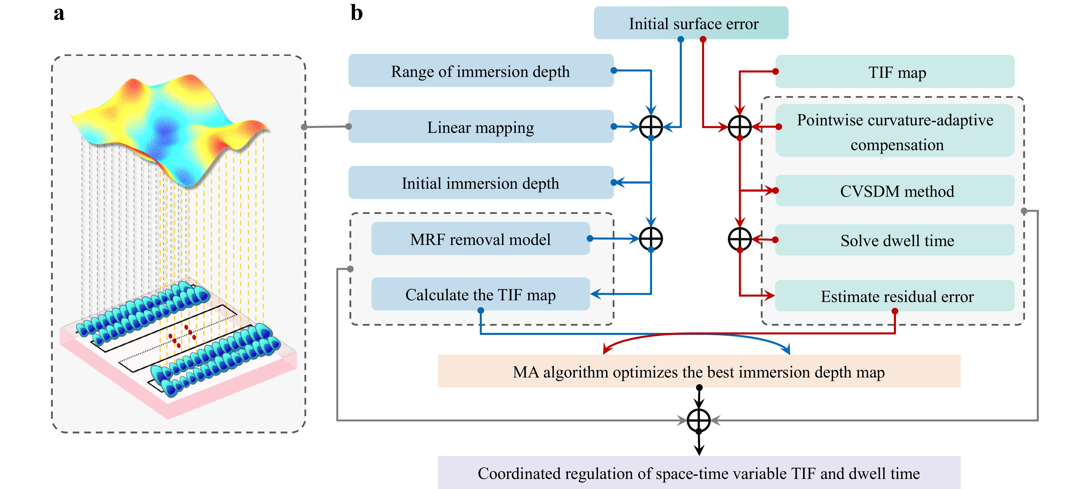
Fig. 6  Illustration of dynamic optimization strategy for immersion depth and scanning speed. a Determination of initial immersion depth. b Dual-degree-of-freedom optimization model.

where H_l0 represents the initial immersion depth, Num_wx and Num_wy represent the row and column dimensions of the scanning trajectory matrix, ff(·) represents mapping function, v_min and v_max represent the minimum and maximum scanning speed of the machine, t ^j and $ H_{l}^{j} $ represent the dwell time and immersion depth of the j-th scanning trajectory point, H_lmin and H_lmax represent the minimum and maximum immersion depth of the machine, and ε represents the ultimate resolution of the immersion depth.

Material removal efficiency is governed by immersion depth and scanning speed through a highly nonlinear, multi-parameter coupling, thereby hindering the direct determination of their optimal combination. The ACSV TIF and dwell time obtained from the initially mapped immersion depth may fail to deliver optimal efficiency and accuracy, an adaptive intelligent optimization algorithm is required to adjust immersion depth and scanning speed dynamically.

Genetic algorithms often exhibit limited local search performance³⁶. Particle swarm optimization is influenced by collective behavior, whereas the whale optimization algorithm is more suitable for continuous optimization problems³⁷. Built on the genetic framework, the memetic algorithm integrates local heuristics to enhance solution quality and accelerate convergence^38,39.

The fitness function plays a central role in guiding the optimization process. The root mean square value of residual error (ERMS) quantitatively evaluates the deviation of the manufactured surface from the target morphology. The error convergence rate (ECR) measures the decline in surface error (such as RMS) per unit time, representing convergence efficiency during modification. The total dwell time (TDT) serves as a primary indicator of machining efficiency. The design goal of the optimization strategy should focus on:

where ^* represents the normalized operation.

To validate the proposed multi-spatial-frequency ultra-precision and efficiency-enhanced paradigm based on the dynamic co-variation of immersion depth and scanning speed, both simulations and polishing experiments were conducted on the laboratory-built six-axis five-linkage MRF machine equipped with the linear motors capable of achieving 1g acceleration, as shown in Fig. 7.

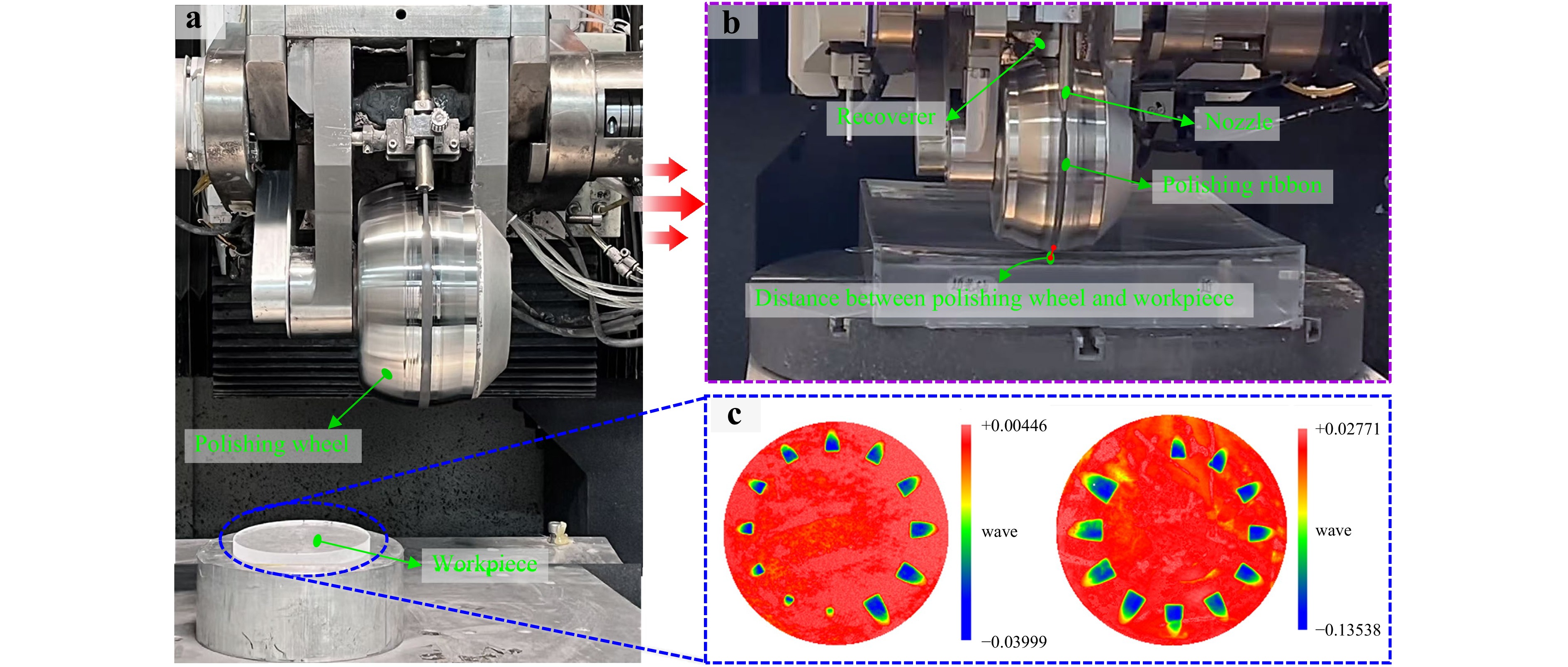
Fig. 7  The experimental machine and the results of the spot experiments. a The experimental machine. b The machine under operational conditions. c MRF TIFs at different immersion depths obtained from the spot experiments.

The MRF TIFs corresponding to immersion depths of 0.05−0.49 mm were obtained through spot experiments on a 100 mm diameter quartz plane mirror, under wheel speed of 260 r/min and processing time of 2s or 8s, employing diamond abrasives, an immersion depth variation rate of 0.02 mm, a wheel radius of 100 mm, a magnetic field current of 10A, and MR fluid containing 82% magnetic particles. Subsequent simulations and polishing experiments were carried out under identical conditions, with immersion depth as the sole variable.

Fig. 7c shows that the immersion depth of the polishing wheel influences both the profile and efficiency of the TIF, validating the feasibility of employing the ACSV TIF for multi-spatial-frequency error correction.

The TIFs acquisition parameters shown in Fig. 7c were used as model inputs to calculate the corresponding shear stress and pressure. Theoretical fitting yielded the model parameters K = 5.0161⁻¹⁰, α = 0.11907, which were substituted into the removal efficiency model defined in Eq. 7 to construct theoretical TIFs at various immersion depths. The similarity index SIM (defined in Eq. 37) was employed to quantitatively evaluate discrepancies between theoretical and experimental TIFs, with representative error distributions visualized in Fig. 8.

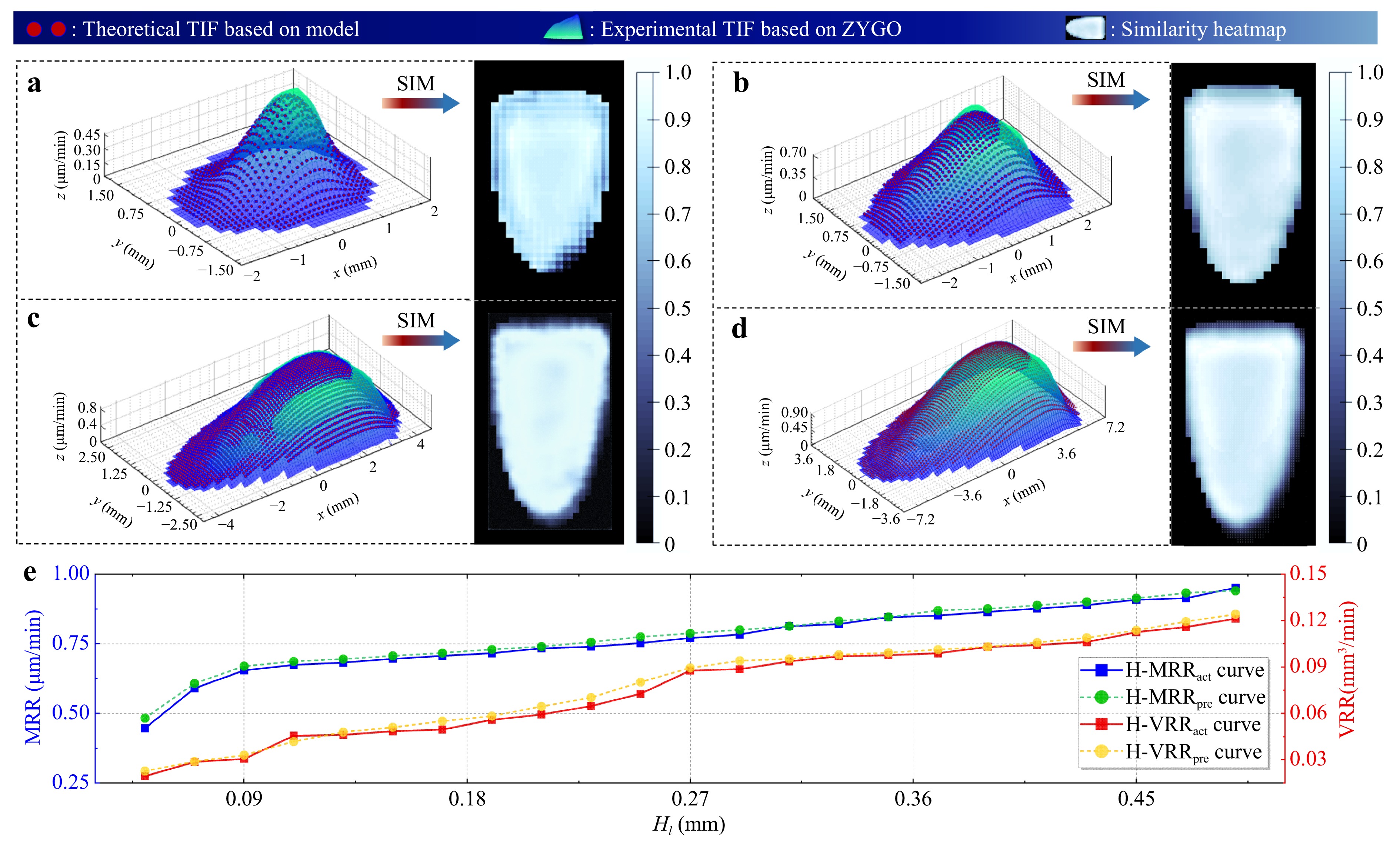
Fig. 8  Accuracy analysis of MRF TIF modeling. a-d TIFs and SIM heat maps at immersion depth of 0.05 mm, 0.13 mm, 0.27 mm, and 0.41 mm. e The predicted and actual comparison curves of MRR and VRR at all immersion depths.

where TIF_E^i,j and TIF_T^i,j represent the values of experimentally measured and the theoretically modeled TIF matrices at the i-th row and j-th column under the same immersion depth, respectively. ε_sim is an infinitesimal constant introduced to prevent the denominator from approaching zero. The computed similarity matrix SIM ranges from 0 to 1, with values closer to 1 indicating higher consistency. The heat map based on SIM is presented in Fig. 8.

Combined with Fig. 8, statistical analysis indicates that across all immersion depths, approximately 86% of the area exhibits SIM ≥ 0.95, with the primary regions approaching a similarity of 1, demonstrating high modeling accuracy and overall consistency. Deviations between modeled and actual results primarily originate from: (1) at TIF edges, rapid spatial variations may amplify measurement noise, machine microvibrations; (2) at TIF edges, the rapid decay of fluid thickness may cause the MR fluid flow to deviate from the ideal laminar assumption, introducing slight deviations; (3) in TIF peak regions, maximal shear stresses induce nonlinear enhancement of material removal, increasing sensitivity to disturbances and structural heterogeneity of the material; (4) minor surface errors may be present in the experimental workpiece used for sampling. Nevertheless, these differences remain minor and have little impact on the overall prediction, without undermining the model's validity and applicability.

To further validate the reliability of the MRF TIF model, immersion depths ranging from 0.05 mm to 0.49 mm were analyzed with a resolution of 0.02 mm, and the predicted and measured maximum removal rate (MRR) as well as volumetric removal rate (VRR) were compared, as shown in Fig. 8e. The results reveal that across all immersion depths, the predicted values are highly consistent with actual data for both maximum and volumetric removal rates. In summary, the SIM heatmaps and removal rate comparisons fully confirm that the model achieves high predictive accuracy, maintaining strong consistency with actual results at different immersion depths, thereby providing robust theoretical support for the strategies based on time-variant tool influence function.

To verify the effectiveness of varying immersion depth for surface error correction, two simulated fabrication paradigms were designed and compared. The first adopted the traditional paradigm, characterized by non-uniform dwell time with a constant TIF, in which the polishing wheel operated at a fixed immersion depth of 0.25 mm. The second employed the ACSV TIF with uniform dwell time. The corresponding simulation results of both paradigms are shown in Fig. 9.

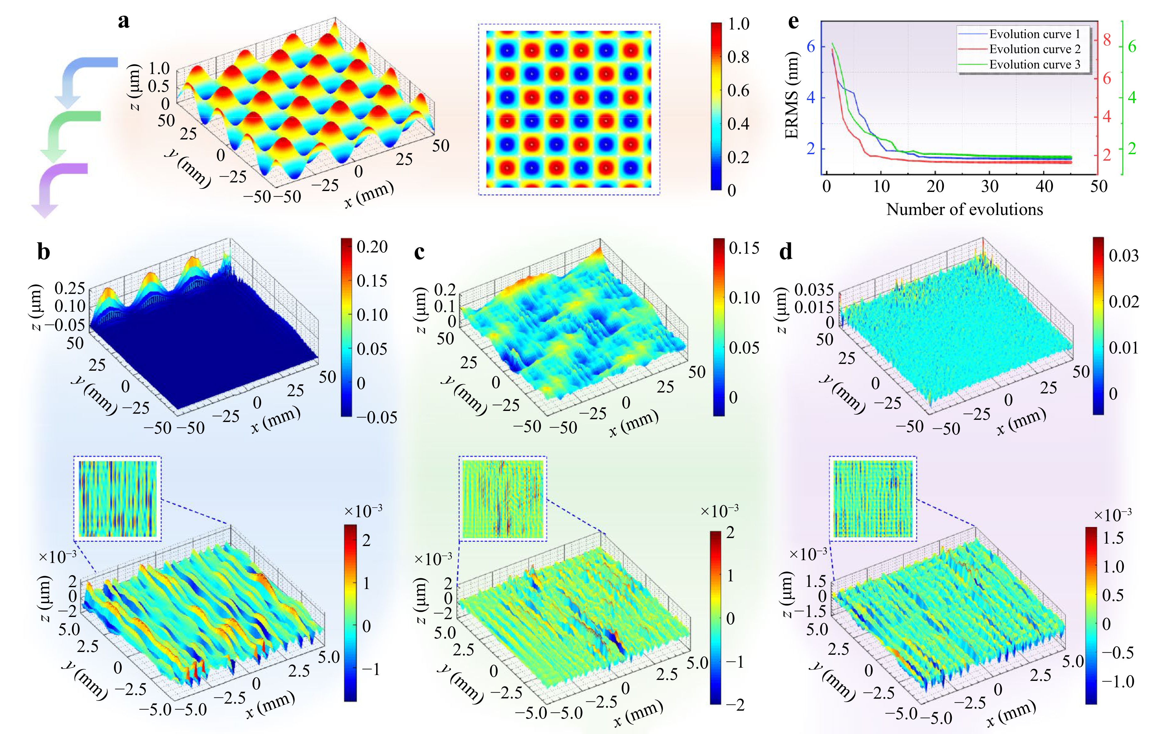
Fig. 9  The simulation results of different paradigms. a Initial surface error. b-d Residual error(up) and MSF error(down) after constant TIF paradigm, dynamic TIF-constant time paradigm, TIF-dwell time covariant paradigm. e Evolution curves.

A comparative analysis of Fig. 9b, c demonstrates that the paradigm employing the ACSV TIF with uniform dwell time effectively suppresses the MSF error. When combined with a constant scanning speed, the TIF exhibits the capability to correct surface errors. However, the immersion depths derived from linear mapping of the initial error fail to achieve optimal accuracy. The constant-speed constraint limits removal efficiency, thereby reducing correction performance.

Previous results indicate both the ACSV TIF and non-uniform dwell time can independently modify surface errors. Building on this, the dual-degree-of-freedom dynamic co-variation model simultaneously coordinates TIF and dwell time to enhance both accuracy and efficiency. Simulation results are shown in Fig. 9d, with error evolution curves in Fig. 9e. Multiple independent runs yield highly consistent outcomes, confirming strong global convergence capability and robustness of the optimization algorithm.

The root mean square (RMS) and the total dwell time are employed to systematically evaluate the manufacturing accuracy and efficiency of three manufacturing paradigms. The corresponding quantitative results are summarized in Table 1.

According to the comprehensive analysis of Fig.9 and Table 1, compared with the variable dwell time modification paradigm under the constant TIF used in traditional sub-aperture polishing, the dual-degree-of-freedom coordinated control paradigm enhances manufacturing accuracy by approximately eightfold and efficiency by more than twofold, while also enhancing convergence of mid-spatial-frequency error. Simulation results confirm that the manufacturing paradigm based on the IDSS-DC model exhibits strong potential for high-efficiency and high-performance optical fabrication.

To further deepen the comparative analysis with the traditional manufacturing paradigm, continuous phase plates exhibiting a complex surface distribution were selected as the experimental subjects. Two CPP workpieces with similar peak-to-valley and RMS values of the initial errors were chosen.

The dwell time for workpiece1 was calculated using the variable dwell time modification paradigm with a constant TIF, resulting in a total dwell time of 456 minutes. Fabrication of workpiece2 employed the dual-degree-of-freedom coordinated control paradigm. Immersion depth distribution was optimized to minimize ERMS and maximize processing efficiency, with a total dwell time of 309 minutes.

Comparative analysis of Fig. 10a, b, as well as Fig. 10d, e, reveals that the dual-degree-of-freedom coordinated control paradigm achieves nearly a 10% higher RMS convergence ratio in single-pass fabrication compared with the traditional approach. Analysis of Fig. 10c, f further indicates pronounced improvement in MSF error convergence. Experimental results confirm that the immersion depth-scanning speed dynamic co-variation paradigm increases efficiency by approximately 32% while maintaining nanoscale accuracy and improving overall manufacturing performance.

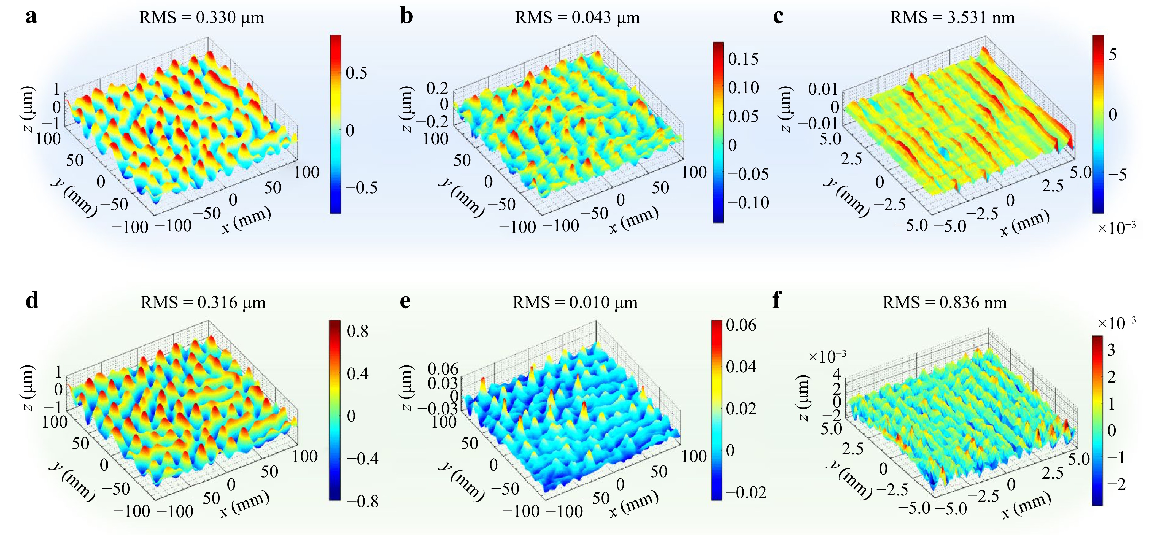
Fig. 10  The actual fabrication results of different manufacturing paradigms. a-c Workpiece 1: initial surface error before polishing, residual error and MSF error after constant TIF paradigm. d-f Workpiece 2: initial surface error before polishing, residual error and MSF error after dynamic TIF-constant time paradigm.

A high-precision optical manufacturing paradigm has been systematically established through the co-evolution of TIF removal efficiency and profile. An actively controllable spatiotemporally variable TIF was implemented, and an innovative dual-degree-of-freedom modification strategy coordinating TIF and dwell time was constructed. A theoretical TIF model was developed to analytically reveal how synergistic variations in efficiency and profile enhance the convergence of mid-spatial-frequency error. Furthermore, a constant-variable speed dual-mode dwell time solution was proposed to maximize removal efficiency, and an immersion depth optimization approach was formulated with consideration of error morphology and manufacturing constraints. Both simulations and experiments confirm that the two-degree-of-freedom paradigm surpasses the traditional constant-TIF paradigm in correction accuracy, MSF error suppression, and manufacturing efficiency. The findings provide a solid theoretical foundation and practical framework for advancing ultra-precision, multi-spatial-frequency error cooperative convergence, and high-efficiency optical fabrication.

The presented work was funded by National Natural Science Foundation of China (62375019), National Key Research and Development Program of China 2021YFC2202403-2. The authors acknowledge the financial support.