Various technologies for the testing of asphere and freeform optics and their calibration

The century of the photon is unthinkable without components that transport, shape, and adapt light for its manifold applications. The production of optical components necessitates metrology that is capable of supporting the manufacturing process, as the iterative nature of production would not converge without it. Optical surfaces with low symmetry (i.e., aspheres and freeform surfaces) pose a particular challenge. The last few decades have seen a significant push in the development of form metrology technologies for those surfaces, as progress in manufacturing with ultra-high-resolution polishing technologies - such as ion beam figuring or magnetorheological finishing - is currently limited by metrology capabilities. In addition to achieving a low measurement uncertainty and the flexibility to measure as wide a range of specimens as possible, the current focus is on reducing measurement time, as this is ultimately the key to cost-effectiveness. If we restrict ourselves to measurement times less than a minute for a full-field measurement, few options remain: Sequential coordinate measuring approaches, e.g. using systems like the ISARA400 of IBSPrecision¹ or the NPMM200 developed at TU Ilmenau² have long measurement times, typically ranging from below an hour to many hours. Faster point-scanning machines include an optical probe and at least one rotation axis to take advantage of the rotational symmetry of aspheres, allowing for full surface scans to be completed in the range of 5 to 15 minutes. Examples of such instruments include the MFU200 of Mahr^3,4, the LuphoScan260 by Taylor-Hobson⁵ or the NANOMEFOS⁶ machine, which was originally developed at TNO and is now commercialized by Dutch United Instruments. Naturally, the measurement time is highly dependent on the scan path, the resulting point density, and the size of the surface under test (SUT).

Much shorter data acquisition times can be achieved with camera-based systems. Incoherent, gradient-based techniques, such as phase-measuring deflectometry (PMD), prove to be flexible and fast, yet their form measurement accuracy is somewhat limited due to the inherent requirement of numerical integration. Burke states in his review paper on deflectometry a typical minimum shape uncertainty in the range of some 100-200 nm for flat or weakly curved surfaces⁷.

Areal interferometry easily achieves nanometer resolution and therefore was used as early as around 1810 by Joseph von Fraunhofer to assess the quality of the (spherical) lenses he manufactured^{8, 9}.

The scope of this paper is limited to full-field areal interferometry approaches, which measure the SUT as a whole, i.e. without relative positioning between the SUT and the interferometer during measurement. Therefore, methods such as stitching¹⁰ and scanning^{11, 12} interferometry are not considered here.

What we want to keep in focus is the topic of calibration.

The interferometric null test is state of the art: The test wavefront of the interferometer is adapted to the test specimen using a so-called null optic system, which leads to retroreflection of the test rays and therefore to a null interferogram for perfect SUTs. This approach avoids retrace errors, i.e. wave front errors introduced by the optical system for rays that do not travel along the calibrated paths. However, since the null optic is an integral part of the interferometer cavity, it introduces systematic errors that need to be calibrated.

In a null test, the calibration function $ W $ is twodimensional:

$ n $ and $ m $ being the pixel coordinates of the interferometer.

Symmetries of any kind enable absolute testing. The term absolute indicates that there is no need for and dependence from a third party reference such as transfer artifacts commonly used to establish traceability to the international unit system. Instead, symmetries allow to separate SUT topography from systematic errors based on a sequence of measurements at different positions and/or multiple orientations. Prominent examples include the three-flat method^14-16, random ball test¹⁷, the Jensen 3 position test for spherical surfaces¹⁸. The latter can be adapted to cylindrical surfaces also¹⁹. Yang suggested a two step shift-rotation method for the calibration of spherical surfaces²⁰. Symmetries in one dimension can also be exploited. For istance, the angular averaging method can be applied to determine non-rotationally symmetric errors of aspheres²¹ or other components of an optical null setup, such as the non-symmetric error of a CGH²². Bloemhoff suggested a method using small lateral shifts between measurements followed by integration²³. The resulting absolute measurement procedure is suitable for flats and spheres and was later adapted to axicon¹³ (cf. Fig. 1) and cylinder surfaces^{24, 25}.

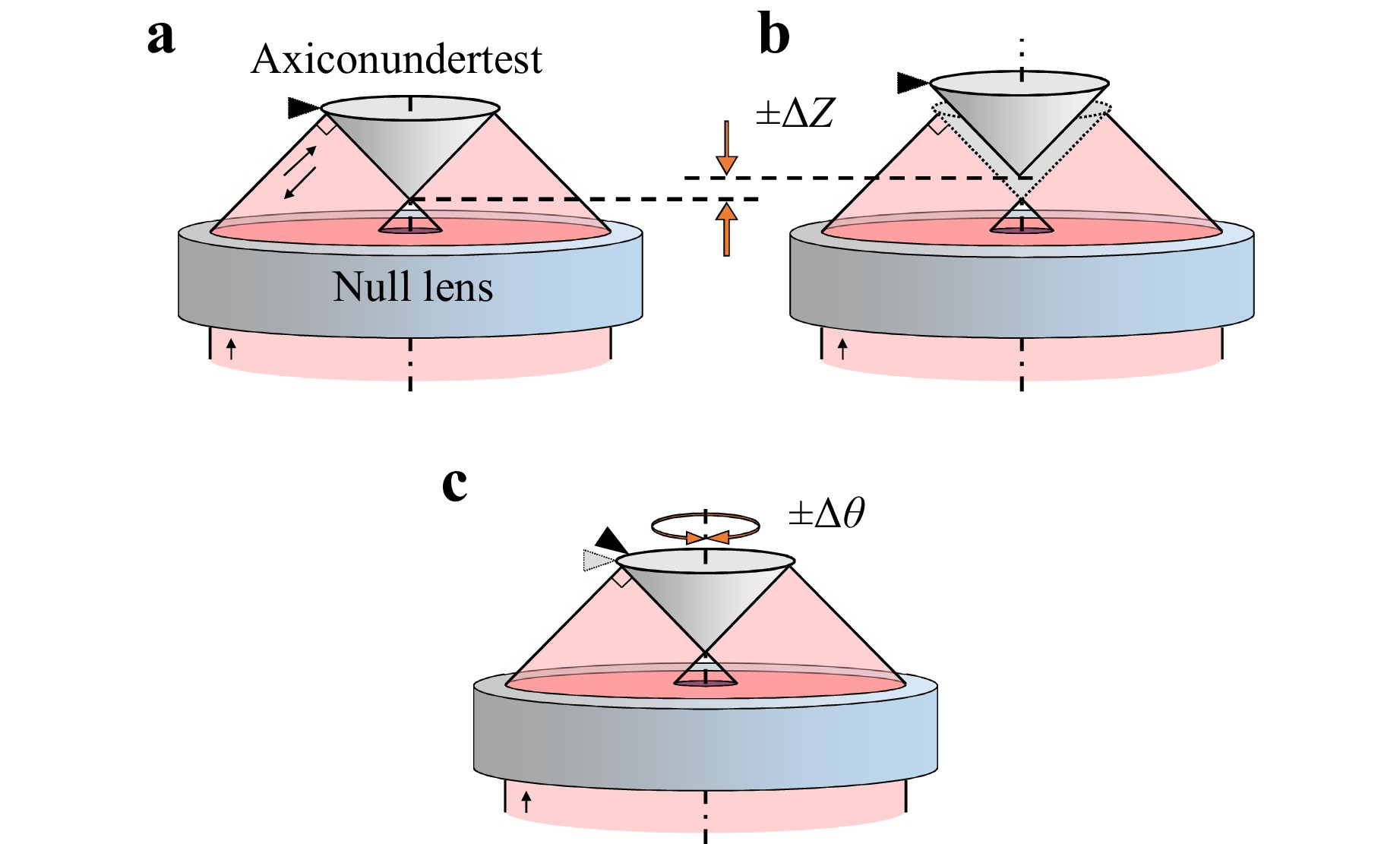
Fig. 1  Absolute test of axicon surfaces exploiting rotational and translational symmetry of the SUT. Three measurements are necessary: a Test setup illuminating the axicon from below using a null lens, b shift along axis of rotation and c rotation. Adopted from Ref. 13.

By definition these approaches are unsuitable for general freeform testing due to the inherent lack of symmetry in such surfaces. However, principles like translational and temporal invariance can still be used to assess uncertainty, e.g. in round-robin experiments, or to check plausibility under certain assumptions²⁶.

Computer-generated holograms (CGH) are state of the art null optics because of their almost unlimited design freedom, including auxiliary features in subapertures and the simultaneous reconstruction of multiple wavefronts, high quality fabrication with lithography equipment and their - compared to refractive null optic systems - moderate price and short lead times. They were first proposed by MacGovern, Wyant and Lohmann in the early 1970s as null optics for the measurement of aspheres^27,28 and since then steadily developed alongside advancements in fabrication and design capabilities^29-31.

The ability to integrate alignment structures is utilized intensively, especially for measuring freeform optics and in large test setups^32-35.

CGH errors originate from substrate form errors, microstructure displacement errors and microstructure errors. The displacement error $ {\boldsymbol{\zeta}}(x,y) $ leads to phase errors $ W_{PD}(x,y) $ in the reconstructed wavefronts of the CGH according to the formula³⁶:

where $ \lambda_0 $ is the design wavelength, $ m_R $ the reconstruction order, and $ {\boldsymbol{\nu}}(x,y) $ the local line density - a vectorial quantity that points perpendicular to the grating lines.

Displacement errors have been calibrated based on fiducials and fabrication monitoring^{37, 38}, microstructure errors have been addressed through diffractometric microstructure characterization^{39, 40}. The effects of substrate errors can be minimized by integrating the reference surface of the interferometer into the CGH structures. In these Diffractive Fizeau Null Lenses (DFNL)⁴¹, only the surface flatness of the CGH side contributes to the systematic error.

In 1993, Burge proposed calibrating refractive null optical systems by replacing the SUT with a CGH⁴², taking advantage of the high quality of the reconstructed wavefront. Recently, a similar approach for calibrating a null test setup using a diamond-turned calibration element was reported⁴³.

Reichelt further developed the concept of a diffractive calibration element to account for potential errors within the CGH itself. The key is to encode auxiliary wavefronts into the CGH that can be directly measured, allowing to predict the CGH's total wavefront error^44,45. Fig. 2b shows a CGH that demonstrates this principle⁴⁶.

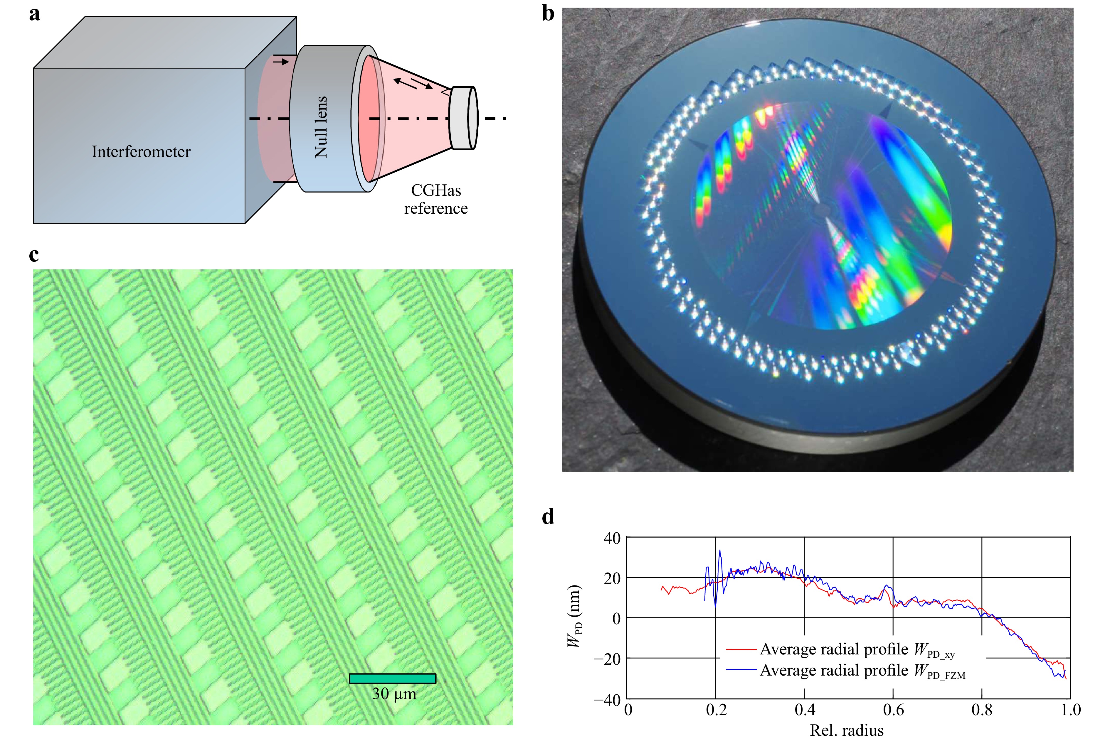
Fig. 2  a Schematic of a triple-CGH used to calibrate a null test setup. b Photo of a triple-CGH with a substrate diameter of 90 mm. c Microscopic detail of the subaperture encoding to reconstruct three wavefronts. d Comparison of the measured (blue) and reconstructed (red) average radial profile.

The CGH multiplexes a Fresnel zone plate (FZP) and two orthogonal linear gratings. The underlying principle is that all structures experience the same displacement error $ {\boldsymbol{\zeta}}(x,y) $. The displacement error is a vectorial quantity that describes for each point the direction and displacement distance caused by positioning inaccuracies while writing the CGH. Each of the linear gratings reconstructs nominally plane wavefronts that carry the signature of the displacement errors, as described by Eq. 2. By measuring all four auxiliary wavefronts reconstructed by the linear gratings in complementary orders under their respective Littrow condition, i.e. in null testing condition, the error of the FZP can be predicted from the displacement error according to Eq. 2, the substrate error and the microstructure errors.

Each of the linear gratings reconstructs complementary diffraction orders $ m_R=\pm 1 $. Using these complementary orders allows for the separation of substrate errors from displacement errors, because the sign of $ W_{PD} $ reverses with the diffraction order $ m_R $⁴⁴.

Fig. 2 compares the measured wavefront error of the FZP to the prediction derived from the measurements of the auxiliary wavefronts, both presented as averaged radial profile. They show good agreement, except in the center region. In this area, overlapping diffraction orders cause significant deviations, highlighting a key limitation of the measurement technique.

The triple-CGH approach determines the complete vectorial displacement function and therefore can be used to calibrate arbitrary CGH. Since it is the holographic counterpart of the surface under test, the same alignment tolerances apply. A major advantage of CGH in general is the possibility to integrate alignment structures like fiducials and retroreflecting elements such as linear gratings or diffractive spherical mirrors. In principle, a triple-CGH can replace any freeform in a null testing setup, including highly irregular ones. Even though it is advantageous in terms of straylight generation and diffraction efficiency to position the CGH outside any caustic region, Su et al. have demonstrated that CGH can also be designed to work there⁴⁷. However, there might be fabrication limitations regarding CGH size for very large freeforms, since the required CGH dimensions generally scale with the size of the freeform under test. Also, steep gradients of the freeform require high line densities in the triple-CGH that might challenge fabrication and also design capabilities⁴⁸.

The considerations made so far have been limited to null testing, which by design suffers only minimally from retrace errors. Flexible testing, which does not rely on individually fabricated and calibrated null test settings leaves these solid grounds, with few exceptions. One such exception is the aforementioned subaperture metrology, which uses mechanical scanning or stepping. Here, positioning errors add uncertainty. Another approach uses the wavelength to obtain the required flexibility, e.g. using diffractive elements with their excellent calibration properties in combination with a variable illumination wavelength⁴⁹.

Flexible testing that requires advanced calibration includes sub-Nyquist interferometry⁵⁰, two-wavelength interferometry used by Wyant to reduce sensitivity⁵¹ or multiple wavelength interferometry, which uses the same setup at different wavelengths to obtain varying incidence conditions on the SUT⁵². Multiple wavelength interferometry can also increase the unambiguity range to extend the capabilities of Fizeau interferometry. With high resolution cameras, optimized interferometer design and a scanning wavelength detection, Stašík was able to measure aspheres with more than 230 µm of aspheric deviation without using null optics⁵³.

In flexible testing, the calibration function becomes dependent on the raypath and, therfore, on the surface under test:

where $ a_{SUT} $ symbolizes the parameters of the SUT in the most general way, including position and orientation information.

However, these methods are limited by vignetting, i.e. the loss of parts of the returning wavefront at lens mounts or the interferometer aperture. Their flexibility primarily stems from the detection, with basically no changes applied to the illumination side. The concept of partial null lenses adapt the illuminating wavefront to the SUT, but accepts non-perpendicular incidence onto the surface. Early approaches with only one lens were introduced by Ross⁵⁴ or the classic two-lens test setup for parabolic and hyperbolic mirrors presented by Offner in 1963⁵⁵. Movable plate systems that can be adjusted to different test specimens have also been proposed^56-58, as well as new types of components like adaptive mirrors⁵⁹ or spatial light modulators⁶⁰. The challenge these systems impose is the calibration of the setup. The calibration function becomes dependent on the raypath through an adaptable partial null system and on the surface under test:

where $ a_{PN} $ symbolizes the parameters of the partial null system in the most general way, including reconfiguration information. In principle, the difficulty to measure the SUT is transferred to measuring the null corrector setup. The commonly applied strategie is to use only a few, simple optical components that are individually characterized and modeled in a raytracing software^{58, 61}. Reconfiguring of the partial null as required for flexible testing necessitates some form of recalibration, since positioning remains a challenge, especially for fast systems, see e.g. Li's discussion on a Hindle sphere test³⁵.

This motivates systems that avoid moveable parts (apart from the SUT) to simplify calibration yet still provide an extended range of illumination to avoid vignetting. MArS, a shearing-based method by Müller and Falldorf ⁶² uses a monolithic array of incoherent light sources with a shearing-based evaluation that measures ray directions and from there reconstructs the shape.

Tilted wave interferometry (TWI) uses a similar strategy to avoid vignetting, but measures interferometric height information instead of ray directions⁶³. The basic idea was developed by Liesener in 2006⁶⁴: In TWI, the SUT is illuminated from different directions (see Fig. 3), e.g. from an array of point sources. The gray cone in Fig. 3 indicates the ray directions that will pass the interferometer aperture. Rays pointing outside the cone will be vignetted. Depending on the local gradient of the SUT, one or the other wavefront will be reflected through the aperture. Since all rays are impinging onto the SUT at the same time, the gradient of the SUT can vary in a large range (typ. ±5°) and still one of the wavefronts is reflected back. As a result, a system of interferogram patches is generated by the mutually tilted wavefronts, covering the whole area of the SUT on the camera simultaneously and can be registered and evaluated.

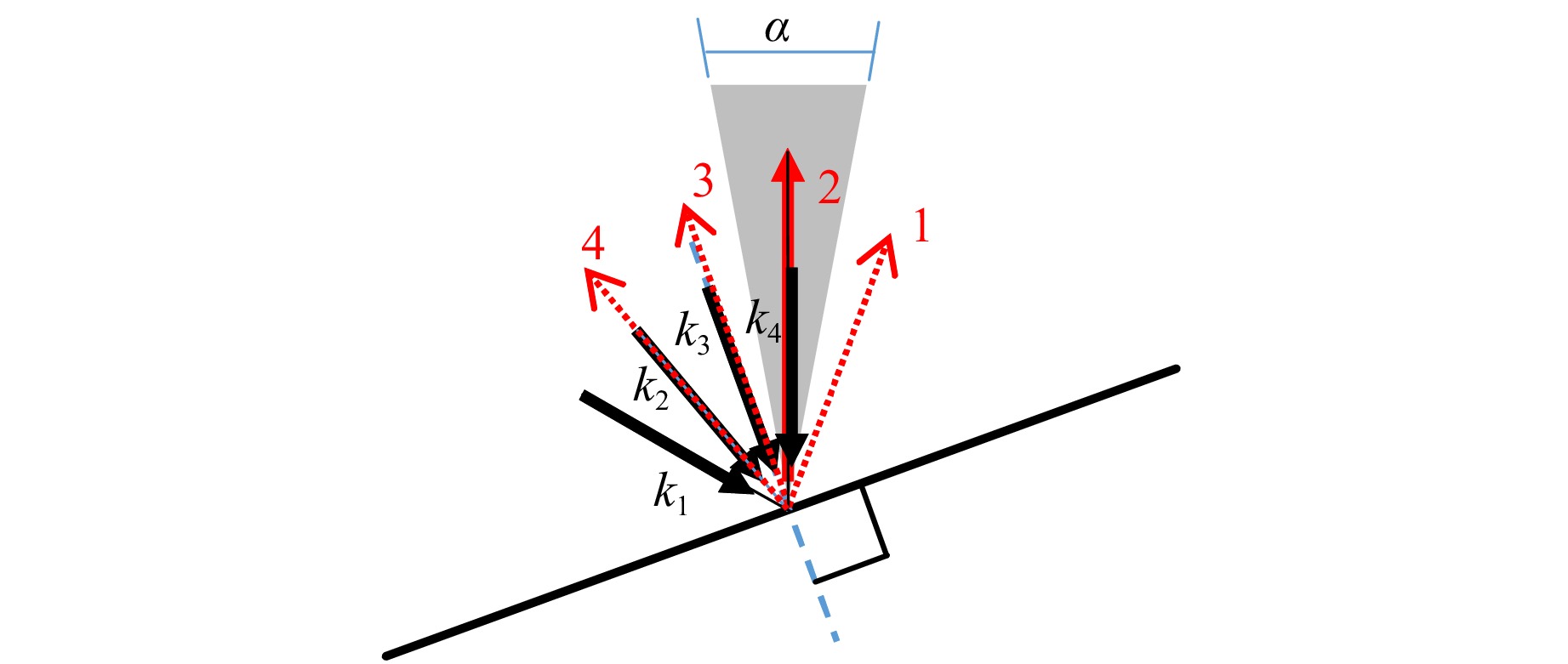
Fig. 3  TWI operating principle: A set of wave fronts, represented by their wavenumber vectors $ k_1 ... k_4 $, impinge onto a point of the test specimen surface and are reflected there. Only one of them reaches the detector, here number 2. The dotted beams are vignetted at the interferometer aperture. $ \alpha $ is the acceptance angle for the angular spectrum.

Naturally, the evaluation needs to remove systematic errors generated by all the retrace errors:

with $ a_{illumination} $ being the influence of the different illumination raypaths.

The calibration task is to explicitly determine this calibration function in order to calculate the quantity of interest - the deviations of the SUT from its nominal design - from the raw measurement data. To illustrate the magnitudes involved: The system calibration function describes the non-null interferograms that are observed at the camera if a perfect SUT is measured. Typically, this means hundreds of wavelengths departure from null test. Any error in the system calibration function will manifest as an error in the SUT measurement. Baer developed the numerics behind it, see also⁶⁵: It is useful to not resort to an explicit digital twin based on lens data and raytracing, but instead introduce a black box system. Here, we only sketch the idea behind the algorithms (see Fig. 4): The SUT is positioned somewhere in the measurement volume. Light from the interferometer (the tilted wavefronts) reaches the surface, gets reflected and propagates through the imaging system to the camera. Since we are only interested in the ray paths in the measurement volume, we introduce two black boxes Q and P that return optical path lengths for a given position and direction. They each refer to a plane in the measurement volume, the source plane $ E_Q $ and the pixel plane $ E_P $. The optical path length $ W_Q $ returned by Q, the source black box, is the path length from a given point source to a given point on $ E_Q $. The optical path length $ W_P $ returned by P, the pixel black box, is the optical path length from a given camera pixel to a given point in the pixel plane $ E_P $. The total optical path length detected on the camera is given by the sum of these segments

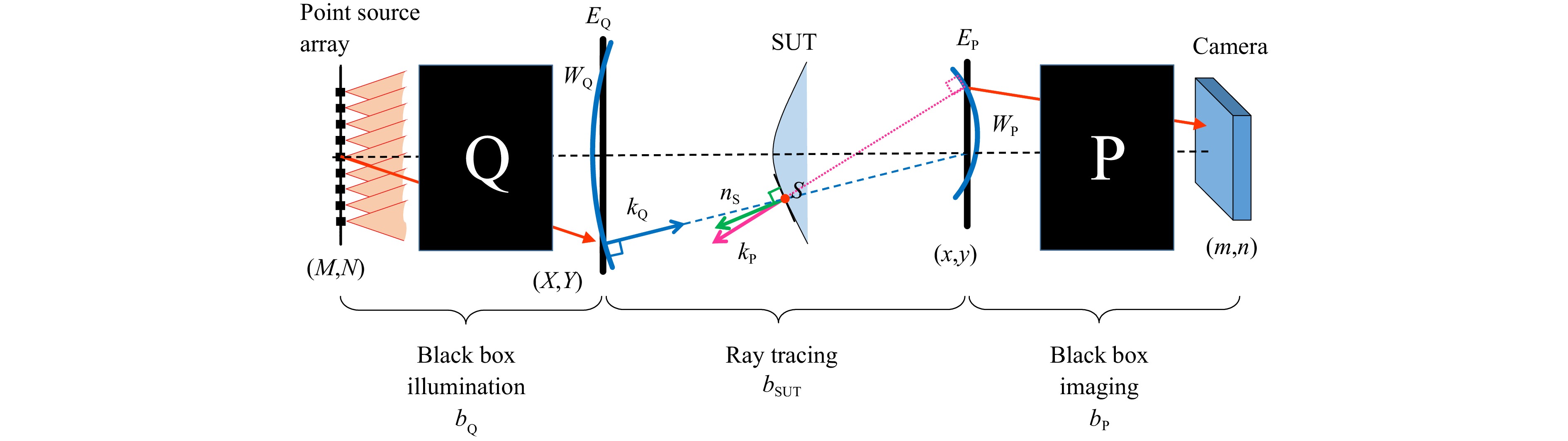
Fig. 4  TWI black box model. Black box Q models the optical path lengths OPL $ b_Q $ of all light rays, emerging from the point source array and ending in the source reference plane $ E_Q $. Black box P models the OPL $ b_P $ of rays from the pixel reference plane to the camera. Between the two black boxes, the OPL are determined using ray tracing.

$ W_{SUT} $ is obtained using raytracing from $ E_Q $ to the SUT, reflecting according to the law of reflection and propagating to the pixel plane $ E_P $. $ N $,$ M $ are the source coordinates, $ n $,$ m $ the pixel coordinates and $ x,y $ the coordinates in the measurement volume.

The implementation of the black boxes are nested Zernike polynomials $ Z $ and describe the optical pathlengths as function of positions ($ X,Y $ resp. $ x,y $) and directions ($ N,M $ resp. $ n,m $):

with the Zernike polynomial coefficients $ Q_{ij} $ and $ P_{kl} $.

The calibration task is to determine the optimal Zernike polynomial coefficients⁶⁶. The number of polynomial coefficients is kept low - typical values are some hundred terms for each Q and P. More terms describe the system calibration function more accurately, less terms improve the numeric stability of the calibration process. Since the polynomial-based description is intrinsically low pass filtering, the effect of camera noise is typically not a limiting factor for the determination of the calibration function.

Important aspects in precision metrology and calibration are mechanical drift and wavelength stability. Calibration CGH incorporate their calibration function in the CGH artifact, which reduces the effects of drift to the temporal invariance of the CGH. Wavelength instabilities, however, introduce a linear error that increases with the number of lines encoded into the CGH. Symmetry-based calibration methods allow compensating schemes to be applied for the required sequence of measurements, mitigating the effects of drift and wavelength instabilities. For flexible measurement approaches, the calibration function of the test setup needs to show temporal invariance both for drift effects as well as for wavelength stability on a time scale exceeding the time between calibration and measurement, which is achieved by proper mechanical and optical design⁶⁷.

Uncertainty estimation of volume calibration methods remains a challenge. Standard tools are Monte Carlo approaches based on digital twins of the interferometer measurement and calibration. Marschall successfully applied a Bayesian uncertainty evaluation on the inverse problem evaluation method of TWI⁶⁸.

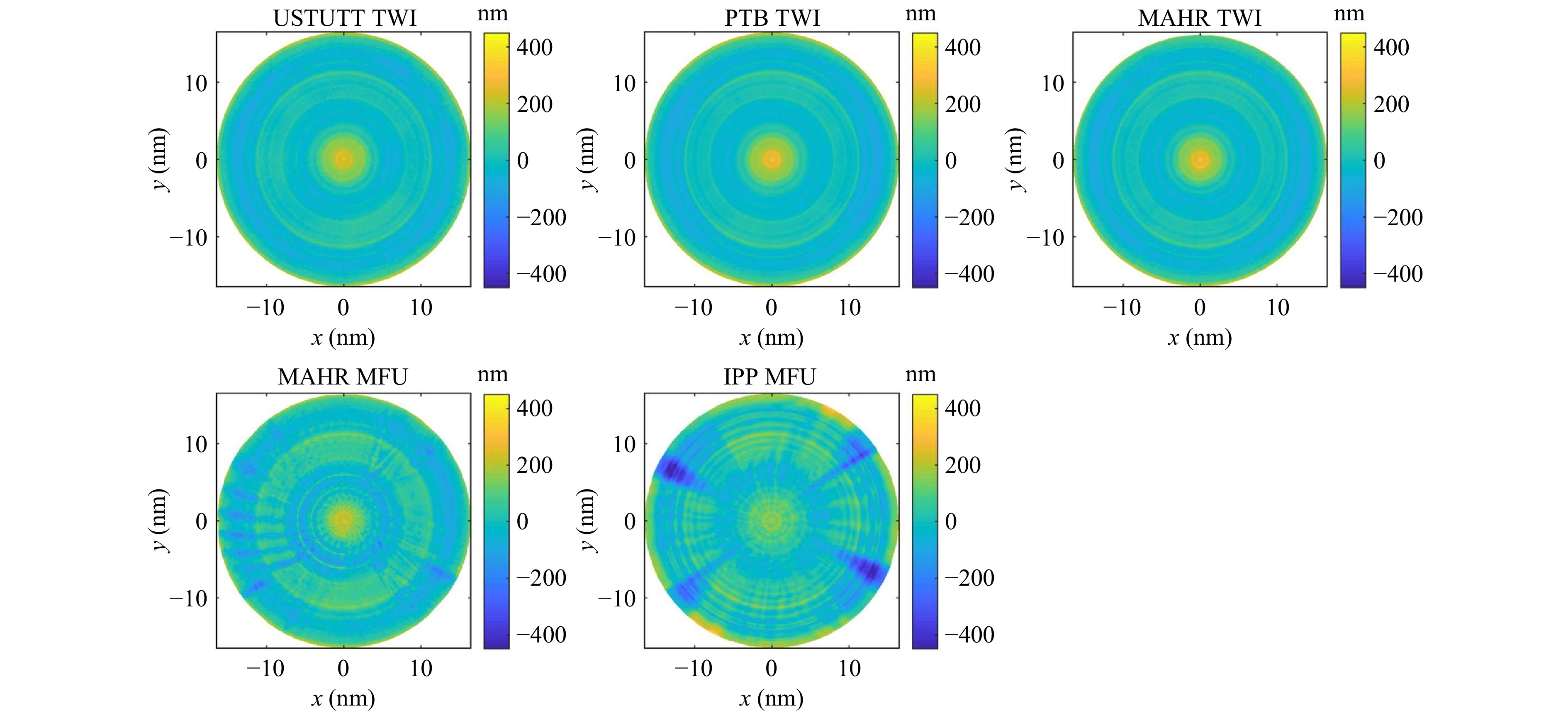
The evaluation of uncertainty at low uncertainty levels relies on comparison measurements, especially in asphere and freeform metrology due to the lack of available calibration specimen. The association CC UPOB e.V. organizes round-robin comparisons and dedicated conferences to address this issue. Results of these activities have been published in two papers^{71, 72}, showing a snapshot of current metrology capabilities.

Fig. 5 shows the results of another round-robin campaign published in⁷⁰. Two tactile instruments and three TWI systems measured the same freeform specimen. The SUT, a so called two-radii-specimen, is a metrological freeform designed to exhibit freeform characteristics while also featuring spherical segments that allow for standard interferometer measurements. The results show close agreement among the TWI instruments involved, suggesting a good performance of the volume calibration function of each instrument.

Fig. 5  Round-robin measurements on a mild metrological freeform surface⁶⁹. Depicted are the deviations from the design form after subtraction of an individual best-fit sphere. Three different TWI setups in three different locations (top row) show very similar results. From Ref. 70.

The separation of the unavoidable systematic errors of an interferometric test setup from the errors of the test specimen to be measured is an integral part of any high-precision measurement. In this paper we touched different methods for accomplishing this separation:

● Exploiting symmetry

● Calibration CGH

● Volume calibration

If the surface under test shows symmetries, they can help to separate systematic errors, e.g. on axicon surfaces. While this is not possible with freeform surfaces in a nulltest, translational invariance still can be exploited in non-null testing^{73, 74}.

CGH offer the design freedom to introduce symmetries for calibration using auxiliary wavefronts. We have shown that with the help of auxiliary wavefronts it is possible to calibrate the reconstructed design wavefront. The method is not limited to any symmetry, so arbitrary freeform wavefronts can be reconstructed, which makes it suitable to calibrate virtually any null optic setup as long as the required line densities remain within the CGH fabrication limits. A comparison of the direct absolute measurement of the reconstructed wavefront with the calibration wavefront prediction calculated from the measurement of the auxiliary wavefronts reveals differences in the single-digit nanometer range. These differences fall within the reproducibility of the interferometer used for this experiment. However, there are also disadvantages:

● Ultimately, the uncertainty of focus and astigmatism error estimation is limited by the positioning accuracy (especially tilt angles) when measuring the auxiliary wavefronts. This can be mitigated using high precision position measurements of the microscopic grating structures in at least three points on the CGH substrate.

● The coding of additional auxiliary wavefronts into the CGH generates additional coherent scattered light, which might lead to unuseable areas. Further research work in advanced coding techniques could help to reduce this effect.

● The positioning of the calibration triple CGH in the calibration measurement potentially leads to additional errors that are not detected by the method. This is a principle problem that is encountered in all SUT measurements⁷⁵. This risk can be reduced by adjustment structures that help to center and orient the calibration triple CGH, but cannot be completely eliminated.

In terms of calibration, the real challenge lies in flexible interferometry. Flexible methods do not require an individually fabricated null optic system but accept a deviation from the null test condition, which leads to retrace errors that need to be known and subtracted. Calibration has been approached with different methods by many groups. As an example, TWI combines static multi-angle illumination with the detection of very high-frequency interferograms on the camera chip. This allows to measure asphere and freeform SUTs with several hundred micrometers departure from best fit sphere. As for all flexible methods, calibration is an integral part of the TWI measurement concept: precise knowledge of the system function allows to predict the optical path length differences measured at the camera for a given test specimen at a given location. Analogous to the computer-stored compensator proposed by Servin for sub-Nyquist interferometry, this path length difference can be mathematically removed from the measurement result⁷⁶. Küchel called this an electronic hologram for the legendary Direct100 interferometer from ZEISS⁷⁷. The term electronic hologram describes the calibration function of the TWI in the literal, holistic sense quite well: The entire error function of the interferometer is contained in the TWI calibration function and can therefore be used for any test situation. However, the polynomial description of system error functions comes with a price: Unless the polynomial orders are chosen exceptionally high^{78, 79}, the system error function is low pass filtered. To a certain degree, this can be taken into account with proper specification of the optical components of the setup. Yet future efforts in flexible calibration need to address the trade-off between lateral resolution of the calibration function and numerical stability.

We would like to acknowledge the funding by the Deutsche Forschungsgemeinschaft (DFG) under project numbers 496703792 and 54555282.