Disturbance-introduced interferometry: surface topography metrology beyond vibration isolation and phase-shifting control

Optical interferometry^1–3 is widely used for surface metrology, with phase-shifting interferometry^4–10 (PSI) being considered the ‘gold standard’ for measuring surface form and texture. To achieve increasingly precise measurements, researchers have consistently pushed the boundaries of hardware capabilities and environmental conditions^11–20. This has resulted in an inherent escalation in system complexity and costs. Furthermore, as many of these strategies approach their theoretical limits, further improvements become increasingly difficult to achieve^21–23. Among these challenges, vibration isolation and phase-shifting control have long been the focus of researchers because they directly affect the accuracy and stability of measurements^24–27.

Various passive and active vibration isolation techniques have been employed to reduce the undesired phase difference between reference and test beams^28–31. These strategies suppress transmitted environmental disturbances, but they do not correct phase-shifting errors or completely remove residual perturbations by themselves. Many phase-shifting techniques have also been developed, including mechanical phase shifters^32,33, modulating polarization^14,18, wavelength modulation¹⁶, displacing a grating^34,35, and tilting a parallel plate. For example, Ref. 32 reported a high-precision large-aperture differential confocal-interferometric method that uses the mechanical phase shifting of a heavy-load reference lens to achieve high-stability surface-profile measurements. However, this approach still relies on dedicated phase-shifting hardware and the precise control of a heavy-load reference element, which increases the system complexity and cost. Ref. 36 applied polarization phase shifting to large-aperture dynamic interferometry but also showed that stress-induced birefringence in large optics introduces polarisation aberrations into the measured wavefront. These errors are not inherently removed by the phase-shifting process and, therefore, require additional characterisation and correction. These challenges are particularly severe for large-aperture components^32,36,37, in which longer measurement cavity lengths and larger test surfaces amplify the effects of vibrations and phase errors. Satisfying stringent performance specifications poses significant challenges, often making the manufacturing of such devices impractical.

Spatial carrier techniques^38–40 are resilient to vibrations and do not require sequential phase shifting; however, they sacrifice spatial resolution and may introduce retrace errors because carrier fringes must be generated by tilting the optical elements. Recently, a deep-learning-based high-precision large-aperture single-frame interferometric method was developed⁴¹; it enables rapid surface-profile reconstruction without a phase shifter. Although promising, this method relies on model training using small-aperture measurements and an aperture-expansion system. Therefore, its broader generalisation across different components and system configurations remains to be further validated. Another class of approaches, referred to as model-based PSI^42–51 or self-calibration methods^52–54, is currently considered promising. For example, an advanced iterative algorithm (AIA)⁴⁴ was developed to simultaneously estimate phase distribution and phase steps. Subsequently, an iterative phase-shifting algorithm^48,51 extended this approach to accommodate minor random tilts. Although these methods can adaptively estimate unknown phase shifts, they fail when the disturbance-induced tilt exceeds one wavelength. Therefore, they currently serve only as supplementary tools when vibration isolation is suboptimal and remain dependent on environmental control and precise phase-shifting equipment.

Because vibrations and phase-shifting errors are inherently difficult to isolate completely, we adopt a counterintuitive strategy: rather than suppressing these disturbances, they are exploited. This approach has resulted in disturbance-introduced interferometry (DII). DII harnesses ambient random mechanical disturbances (RMDs), such as structural vibration or deformation, to naturally encode the measured phase information into interference patterns. RMDs are reconceptualised as beneficial excitation signals rather than detrimental noise, thereby eliminating the need for conventional phase-shifting mechanisms or vibration isolation systems. We present a natural phase decoding algorithm (NPDA) for collecting and analysing interferograms under disturbance conditions. By employing a coarse-to-fine approach and iteratively updating decoupled spatiotemporal variables, the NPDA accurately extracts phase information from interference patterns and adapts to significant disturbances. DII enables nanoscale surface-topography measurements.

As illustrated in Fig. 1 and Supplementary Movie S1, DII involves light from a laser passing through a beam-expanding system to a partially reflective reference surface. At this surface, the incident light is split into two portions: the reflected portion serves as the reference beam, whereas the transmitted portion propagates through the measurement cavity, reflects off the test surface, and returns as the test beam. The two beams are then recombined via the beam-expanding system and imaging lens to form interferometric images at the camera plane. RMDs alter the relative positions of the test and reference surfaces by dynamically modulating the optical path difference between the test and reference beams. This process naturally encodes the interferometric images using RMDs. DII captures these disturbance-modulated interferometric images and subsequently analyses them using the NPDA to decode the interferometric phase and reconstruct the test surface topography.

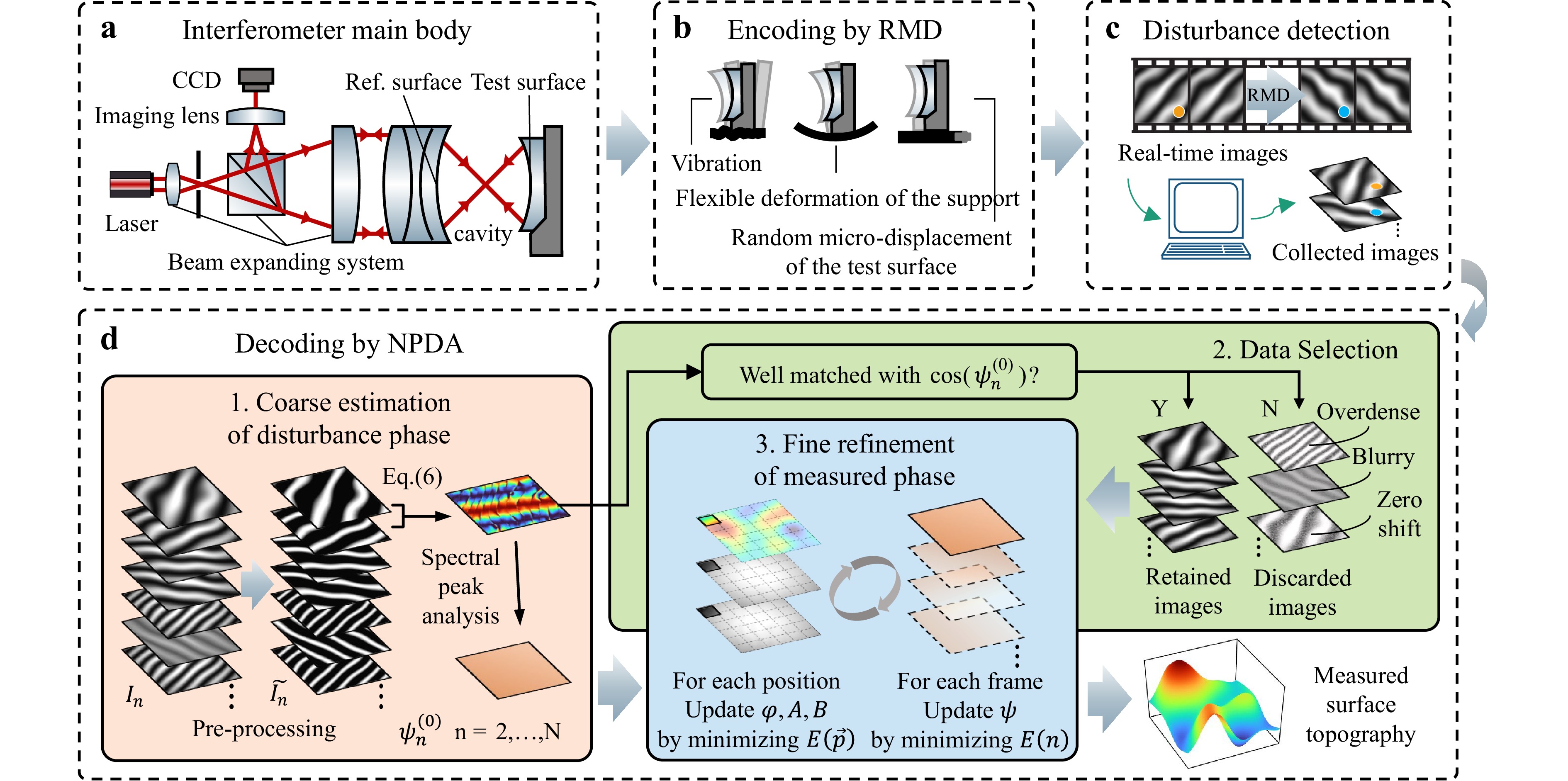
Fig. 1  Schematic of disturbance-introduced interferometry (DII). a Interferometer main body. b Phase information is encoded into the interference patterns via random mechanical disturbances (RMDs), including vibration, support flexible deformation, and random micro-displacement. c Sequential acquisition of interference images under various disturbance conditions. d Extraction of the embedded phase information from the recorded interference patterns through the natural phase decoding algorithm (NPDA).

In DII, RMDs can be introduced passively or actively via vibration, flexible deformation of the support, or random micro-displacement of the test surface. The theoretical interferometric intensity is first described by the standard interference model⁴⁸:

where $ I_{n}^{t}(\overrightarrow{p}) $ is the intensity at pixel $\vec p = (x,{\mkern 1mu} y)$ at time $ n $; $ A $, $ B $, $ \phi $, and $ \psi $ represent the background intensity, modulation amplitude, measured phase, and disturbance-induced phase-shift, respectively. In DII, $ A $, $ B $, and $ \phi $ are considered to be time-invariant, consistent with conventional PSI. Following the widely adopted formulation in tilt PSI^48,51, the disturbance phase is defined as

where $ {d}_{n} $is the parallel phase shift, and $ {k}_{xn},{k}_{yn} $are the tilt gradients along the $ x $ and $ y $ axes, respectively.

To achieve robust performance against significant disturbances while maintaining high precision, the proposed NPDA employs a three-stage coarse-to-fine strategy. In the initial stage, termed the ‘coarse estimation of disturbance phase’, a rapid framewise global estimation of the temporal disturbance variables $ {k}_{xn} $, $ {k}_{yn} $, and $ {d}_{n} $ is performed to obtain their initial values for subsequent refinement. This stage is characterised by the use of spectral analysis to effectively separate the signal from noise. The chirp Z-transform (CZT) is employed to further enhance the resolution of this parameter estimation, enabling a swift yet effective initial assessment. In the second stage, ‘data selection’, a quality control mechanism is implemented to filter the results from the coarse estimation. This process assesses both the interferograms and their corresponding initial estimates, discarding low-quality data and unreliable results. The refined dataset, now comprising high-quality interferograms and reliable initial parameters, proceeds to the final ‘fine refinement’ stage. The spatial and temporal variables are decoupled and iteratively optimised. This optimisation process seeks to minimise the spatial loss function, $E(\overrightarrow{p})= $ $ \sum \nolimits_{n=1}^{N}{\left(I_{n}^{t}(\overrightarrow{p})-{I}_{n}(\overrightarrow{p})\right)}^{2} $, to update the parameters $ A(\overrightarrow{p}), B(\overrightarrow{p}) $, $ \phi (\overrightarrow{p}) $ and to minimise a temporal loss function, $ E\left(n\right)=\sum \nolimits_{\overrightarrow{p}={\overrightarrow{p}}_{1}}^{{\overrightarrow{p}}_{M}}{\left(I_{n}^{t}(\overrightarrow{p})-{I}_{n}(\overrightarrow{p})\right)}^{2} $, to update the frame-specific disturbance parameters $ {d}_{n},\,{k}_{xn},\,{k}_{yn} $. This iterative process is continued until convergence is achieved. Finally, the topographic reconstruction is completed through phase unwrapping and unit conversion of the refined phase map $ \phi $.

Image preprocessing is employed to eliminate the effects of the background intensity $ A $, modulation amplitude $ B $, and phase $ \phi $, yielding an estimated normalized interference image $ {\tilde{I}}_{n}(\overrightarrow{p}) $ that approximates $ \cos \left[\phi (\overrightarrow{p})+{\psi }_{n}(\overrightarrow{p})\right] $.

Here, $ n $ denotes the frame index of the interference image, $ N $ is the total number of images used in the computation, $ {A}_{\text{est}} $ and $ {B}_{\text{est}} $ are the estimated values of $ A $ and $ B $, respectively, and $ \mathrm{LPF}(\cdot ) $ represents a low-pass filtering operation.

For any point $ \overrightarrow{p} $ and its neighbouring point $ \overrightarrow{{p}^{\prime}} $, we assume $ \cos \left({\psi }_{n}(\overrightarrow{p})\right)\approx \cos \left({\psi }_{n}(\overrightarrow{{p}^{\prime}})\right) $. By defining $ {\alpha }_{n}=\cos \left({\psi }_{n}\right) $, the following relationship is derived:

The disturbance phase parameters $ {k}_{xn} $, $ {k}_{yn} $, and $ {d}_{n} $ are then calculated through the following steps:

Here, $ \mathcal{C}\mathcal{Z}\mathcal{T} $ refers to the chirp-Z transform, which enhances the resolution of the initial estimates $ k_{xn}^{(0)} $ and $ k_{yn}^{(0)} $ (see Supplementary Note 1).

Owing to the presence of two conjugate peaks in the spectrum of $ {\alpha }_{n} $, an ambiguity occurs in the disturbance phase parameters across different frames. This is addressed as follows: We define $ {\beta }_{n}=\sin \left({\psi }_{n}\right) $ and compute

where $ \mathcal{W} $ denotes $ 2\pi $-phase wrapping. If

then the parameters are adjusted by setting $ {k}_{xn}=-{k}_{xn} $, $ {k}_{yn}=-{k}_{yn} $, and $ {d}_{n}=-{d}_{n} $ to resolve the ambiguity.

Note that this step only resolves the inter-frame ambiguity, ensuring consistent phase signs across different frames. However, it does not determine the absolute orientation of the measured surface. Resolving the surface sign ambiguity would require additional constraints, such as knowledge of the tilt disturbance direction.

Because our method is based on DII, the occurrence of non-ideal or low-quality interferograms (‘dirty data’) is an expected part of the data acquisition process. These low-quality frames typically fall into two categories.

1. Over-dense fringes: An excessive disturbance amplitude at a given moment can cause the test component to deviate significantly from its ideal position, thereby introducing substantial tracking errors. This manifests as overly dense interference fringes.

2. Blurred fringes: High disturbance frequency can cause the interference pattern to shift significantly during camera exposure, resulting in a blurred image owing to motion artefacts.

To ensure the robustness and accuracy of the final measurements, we introduce a ‘data selection’ mechanism. This mechanism automatically identifies and filters out low-quality frames by evaluating a quality index (QI) of each interferogram. The QI is defined based on the mean squared error (MSE) between the cosine of the estimated disturbance phase $ \cos (d_{n}^{(0)}+k_{xn}^{(0)}x+k_{yn}^{(0)}y) $ and that of the directly computed normalised interference pattern ($ \cos ({\psi }_{n}) $ from Eq. (3)). A higher QI value indicates a better match and thus higher confidence in the data and initial estimate. This mechanism serves the dual purpose of rejecting poor-quality interferograms and filtering out unreliable results from the coarse estimation stage.

The effectiveness of this mechanism was demonstrated in a simulation, shown in Fig. 2. In this example, ten interferograms were processed. Among them, frame $ {I}_{2} $ was synthetically blurred to simulate high-frequency vibrations, whereas frame $ {I}_{3} $ was given a large tilt coefficient to simulate over-dense fringes from excessive displacement. The plot in Fig. 2b compares the calculated QI for each frame with the reciprocal of the ground-truth estimation error (1/Err), where Err is the RMSE between the estimated disturbance phase and its known true value.

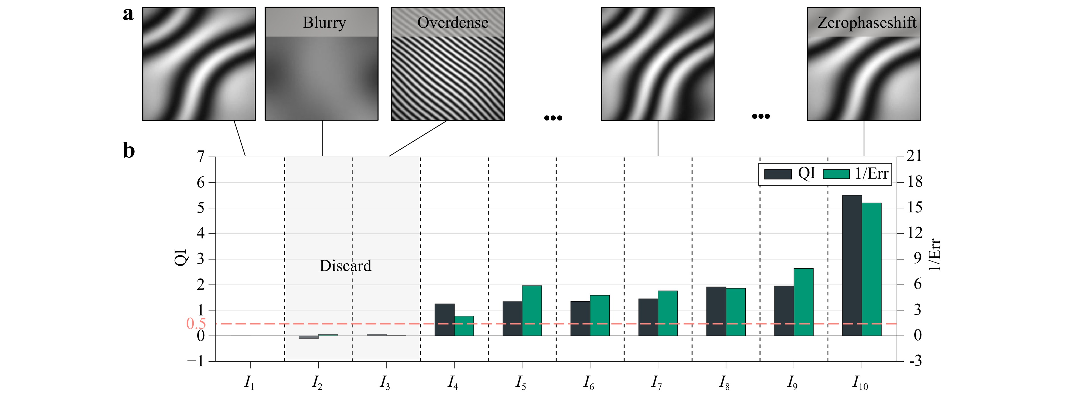
Fig. 2  Validation of the data selection mechanism using the quality index (QI). a Sequence of ten simulated interferograms, sorted by their calculated QI values in ascending order. The set includes deliberately corrupted frames, such as a blurred image ($ {I}_{2} $) simulating high-frequency disturbances and an over-dense image ($ {I}_{3} $) simulating excessive disturbance amplitude. A frame with zero phase shift ($ {I}_{10} $) is also included for comparison. b Plot comparing the QI of each frame against the reciprocal of the ground-truth estimation error (1/Err). The strong correlation demonstrates that the QI is an effective predictor of estimation accuracy. By applying a simple threshold (e.g. QI > 0.5, indicated by the red dashed line), low-quality frames ($ {I}_{2} $ and $ {I}_{3} $) are successfully identified and discarded.

The results clearly showed a strong correlation between the QI and 1/Err, confirming that the QI is an effective predictor of coarse estimation accuracy. By applying a simple QI threshold (e.g. 0.5), low-quality frames with blurry ($ {I}_{2} $) and over-dense ($ {I}_{3} $) fringes were successfully identified and discarded. This validation demonstrated the effectiveness of the data selection mechanism in automatically ensuring that only high-quality data proceeds to the fine refinement stage.

The coarse estimation stage relies on rough approximations, resulting in suboptimal precision that necessitates further refinement. The disturbance phase parameters obtained from the coarse estimation—denoted as $ d_{n}^{(0)} $, $ k_{xn}^{(0)} $, and $ k_{yn}^{(0)} $—and the corresponding disturbance phase $ {\psi }^{(0)} $ serve as initial values for the fine refinement stage.

Because the measured phase $ \phi $ and disturbance phase $ \psi $ are coupled within the cosine function, decoupling them is critical for accurate computation. To achieve this, we employ an iterative strategy separating spatial and temporal variables, consisting of the following two steps, which is an extension of the AIA⁴⁴:

Pointwise update of spatial variables $ A $, $ B $, and $ \phi $

We define $ a(\overrightarrow{p})=A(\overrightarrow{p}) $, $ b(\overrightarrow{p})=B(\overrightarrow{p})\cos \phi (\overrightarrow{p}) $, and $ c(\overrightarrow{p})=-B(\overrightarrow{p})\sin \phi (\overrightarrow{p}) $. The theoretical intensity is expressed as

The loss function is defined as

where $ I_{n}^{t} $ is the theoretical interference image intensity, and $ {I}_{n} $ is the actual acquired intensity. Fixing $ {\psi }_{n}=\psi _{n}^{(t-1)} $ (where $ t $ denotes the iteration round), the parameters $ a(\overrightarrow{p}) $, $ b(\overrightarrow{p}) $, and $ c(\overrightarrow{p}) $ are solved using the least squares method by setting

This can be reformulated as

where

From the solved $\{ R \}$, the updated variables are computed as

After iterating over all pixels, the updated $ {A}^{(t)} $, $ {B}^{(t)} $, and $ {\phi }^{(t)} $ are obtained.

Framewise update of temporal variables $ {k}_{xn} $, $ {k}_{yn} $, and $ {d}_{n} $

The loss function is defined as

Fixing $ A(\overrightarrow{p})={A}^{(t)}(\overrightarrow{p}) $, $ B(\overrightarrow{p})={B}^{(t)}(\overrightarrow{p}) $, and $ \phi (\overrightarrow{p})={\phi }^{(t)}(\overrightarrow{p}) $, the Levenberg-Marquardt (LM) algorithm⁵⁵ within nonlinear least squares is used to iteratively optimise $ {k}_{xn} $, $ {k}_{yn} $, and $ {d}_{n} $. The parameter vector is defined as

The residual is

The Jacobian matrix is

The Hessian matrix and gradient are approximated as $ H={J}^{T}J $ and $ g={J}^{T}r $, respectively. The parameters are updated using

The iterative procedure alternates between updating the spatial variables $ A(\overrightarrow{p}),B(\overrightarrow{p}) $, and $ \phi (\overrightarrow{p}) $ and refining the temporal parameters $ {d}_{n},{k}_{xn} $, and $ {k}_{yn} $ for each frame ($ n= $ $ 2,3,\ldots ,N) $. Convergence in the temporal update is defined by the relative change in the norm of the parameter vector. Specifically, if

where $ {\mathbf{P}}^{(t)}={\left[k_{xn}^{(t)},k_{yn}^{(t)},d_{n}^{(t)}\right]}^{T} $ and $ \epsilon $ is typically set to $ {10}^{-6} $, the iteration is terminated. Otherwise, the process continues until either this criterion is satisfied or the maximum number of iterations (set to 100) is reached. If the criterion is still not satisfied at the 100th iteration, the temporal refinement is terminated, and the current estimate is retained as the output of that update.

To assess the effectiveness of DII, we conducted numerical simulations using MATLAB to model the measurement of a flat mirror. The interferograms were generated according to Eq. (1). Here, the background intensity and modulation amplitude were generated by the function $ A(x,y)=B(x,y)=\exp (\log (0.75)\times ({x}^{2}+{y}^{2})) $. The mirror surface, modelled by $ \phi $, was generated using a peaks function with a PV value of π rad, where the wavelength was 640 nm. The RMD was implemented by simulating the spatial deviations of the test element relative to its ideal position. These deviations encompassed six degrees of freedom, comprising translations and rotations along the x, y, and z axes. For each degree of freedom, the perturbation was modelled as a simple harmonic motion with an amplitude of ±2$ \lambda $ and a frequency of 15 Hz. The simulated camera sampling frequency was 200 Hz. The disturbance phase $ \psi $ was obtained by calculating the offset distance along the optical axis at each sampling instant and applying a unit scaling of $ 4{\text{π}} $/$ \lambda $. Additionally, white noise was incorporated into the interferograms to yield an image signal-to-noise ratio of 40 dB. Under these conditions, the disturbance phase amplitude (DPA)—defined as the maximum PV value of the nonlinear phase shift induced in the measurement cavity (see Supplementary Note 3)—reached approximately 7π rad. This DPA of 7π rad is a typical value under uncontrolled, vibration-prone environments, corresponding to a tilt of 3.5$ \lambda $. For comparison, conventional four-step PSI (4-PSI) was also simulated under two disturbance regimes: strong (DPA = 7π rad) and weak (DPA = 7/100π rad).

The results are shown in Fig. 3, where the DII yielded a remarkably low RMSE of 0.0005$ \lambda $ (Fig. 3a), whereas 4-PSI produced an RMSE of 0.5$ \lambda $ under strong disturbances and 0.006$ \lambda $ under weak disturbances. Notably, even under weak disturbances, the RMSE of 4-PSI was more than one order of magnitude higher than that of DII under strong disturbances. These results underscore the robustness of DII for high-precision surface metrology, maintaining accuracy even when the disturbance levels exceed the tolerance of conventional 4-PSI by more than 100-fold.

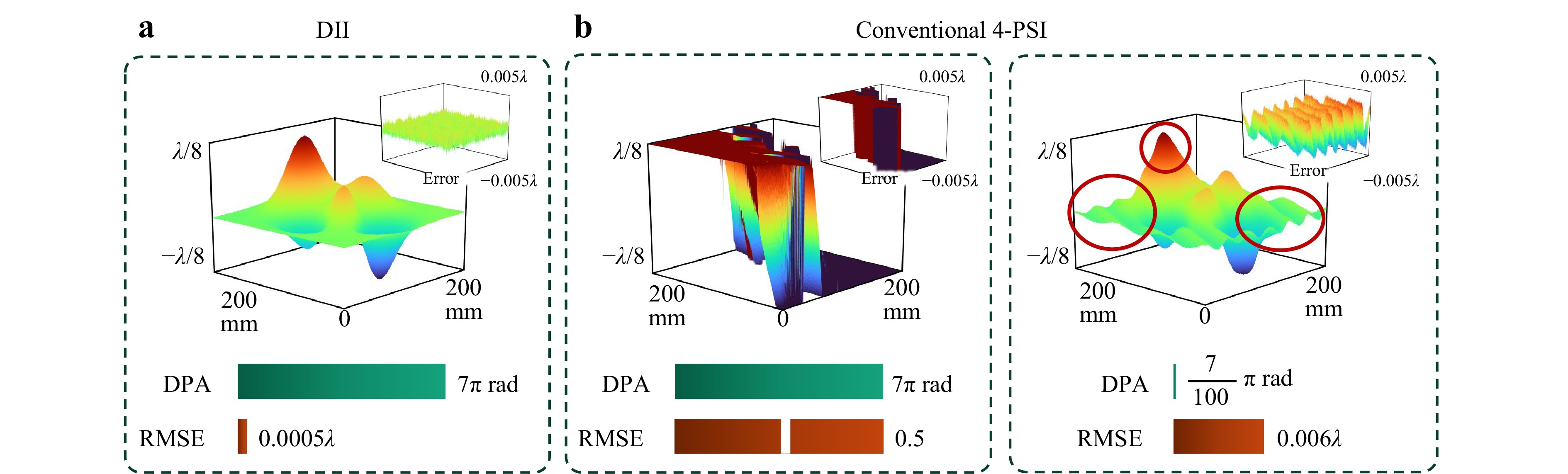
Fig. 3  Numerically simulated surface topography measurements of a planar component. a DII performance under a strong disturbance characterized by a disturbance phase amplitude (DPA) of 7π rad. b Conventional four-step PSI (4-PSI) results under differing disturbance conditions: strong disturbance (left panel) and weak disturbance (right panel, with DPA = 7/100π rad).

We assessed the robustness of the DII method against nonlinear disturbances by testing it across DPAs ranging from 0.01π rad to 12π rad. For comparison, we also evaluated three established anti-vibration techniques widely used in PSI: Hariharan’s five-step algorithm (5-PSI), the AIA⁴⁴, and the general iterative algorithm⁴⁸ (GIA). Test surfaces, with a peak-to-valley height of λ/2, were generated by filtering Gaussian-distributed Fourier spectra. Each test involved five simulated interferograms with nominal phase shifts of 0, π/2, π, 3π/2, and 2π rad, perturbed by random tilts spanning the specified DPA range. Although DII can resolve unknown phase shifts, unlike 5-PSI, we used all methods with ideal phase shifts for equitable comparison.

Performance was assessed using 100 surface samples per DPA level, based on two metrics: the solution success rate (SSR), defined as the percentage of trials where the RMSE of the reconstructed surface was below 0.003$ \lambda $, and the tolerable DPA, the maximum DPA permitting an SSR ≥ 80%. This 80% cutoff was used as an empirical comparison benchmark rather than a physical boundary. This provided a single, moderately stringent criterion for summarising the SSR–DPA curves and comparing the robustness of different methods under the same standard. The main robustness trends were still determined by the full SSR–DPA curves, whereas the tolerable DPA served only as a compact summary metric. These metrics were used to assess the robustness of each method in maintaining reconstruction precision under varying disturbance levels.

As shown in Fig. 4a, DII exhibited exceptional robustness, maintaining an SSR greater than 90% across the full DPA range. Conversely, conventional PSI methods degraded rapidly at lower disturbance levels, with the GIA being the most resilient, failing beyond 0.5π rad. Remarkably, although our tests capped the DPA at 12π rad, the capability of DII likely extends further. However, beyond this threshold, other error sources such as tracking errors would likely dominate the reconstruction, justifying our range limit. This limit depends on the specific system and the measured object. Fig. 4b shows that the tested 12π rad threshold reflected a disturbance tolerance 20 times greater than that of the GIA (0.6π rad) and 120 and 60 times greater than those of the 5-PSI and AIA, respectively. However, subsequent experiments confirmed that a 12π rad disturbance level satisfies practical application requirements.

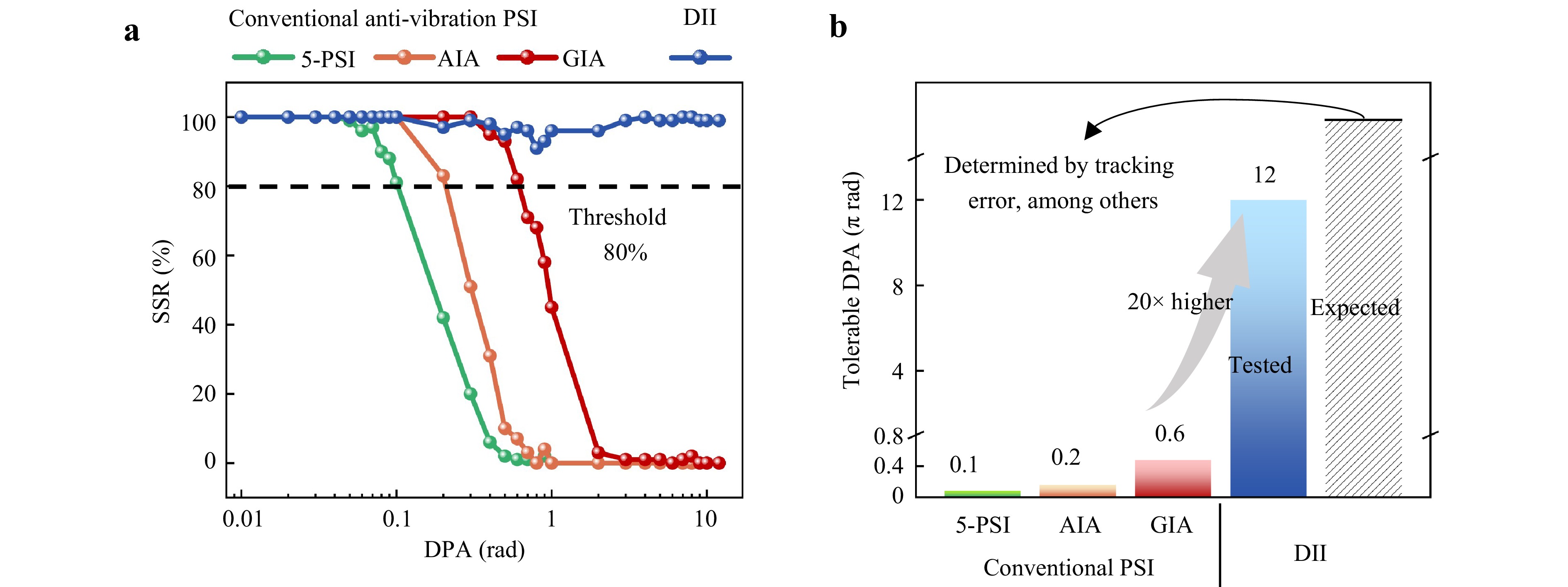
Fig. 4  Robustness comparison of methods under nonlinear disturbances. a Evaluation of the solution success rate (SSR) for the tested methods under DPAs ranging from 0.01π rad to 12π rad. b Assessment of the maximum tolerable DPA for each method.

These findings demonstrate that DII reliably delivers sub-0.003$ \lambda $ precision across a wide range of nonlinear disturbances, where conventional methods become ineffective, extending the practical limits far beyond what was previously achievable by PSI. Among the conventional methods, GIA exhibited the strongest anti-vibration capability. Thus, it was selected as the benchmark for subsequent experimental comparisons.

To validate DII, we developed a Fizeau-type interferometric prototype to measure the optical surface topography. The optical configuration is depicted in Fig. 5a, and the physical setup is shown in Fig. 5b. A 640 nm laser was coupled to an optical fibre (OF), emerging as a divergent beam. This beam passed through a half-wave plate (HWP), stop plate (S), polarising beam splitter (PBS), quarter-wave plate (QWP), plate beam splitter (BS), and large-aperture collimator (LAC) to form a parallel beam. The HWP aligned the polarisation of the beam with the S-polarisation of the PBS for full reflection. The beam split at the reference lens (RL): one part reflected as the reference beam, and the other transmitted and reflected off the tested lens (TL) as the measurement beam. Both lenses were aligned using a precision adjustment mechanism (PAM). Returning light partially entered an alignment module (AAM) for the initial positioning via a charge-coupled device (CCD), whereas the remainder passed through the PBS, reflective mirror (RM), pinhole (P), and small-aperture collimator (SAC). Interference occurred at a rotating ground glass (RGG), captured by a CCD through an imaging lens (IL). All experiments were conducted following a rigorous and standardised internal laboratory protocol, identical to the operational procedures for industry-standard interferometers (e.g. Zygo), to ensure repeatability and validity of the results.

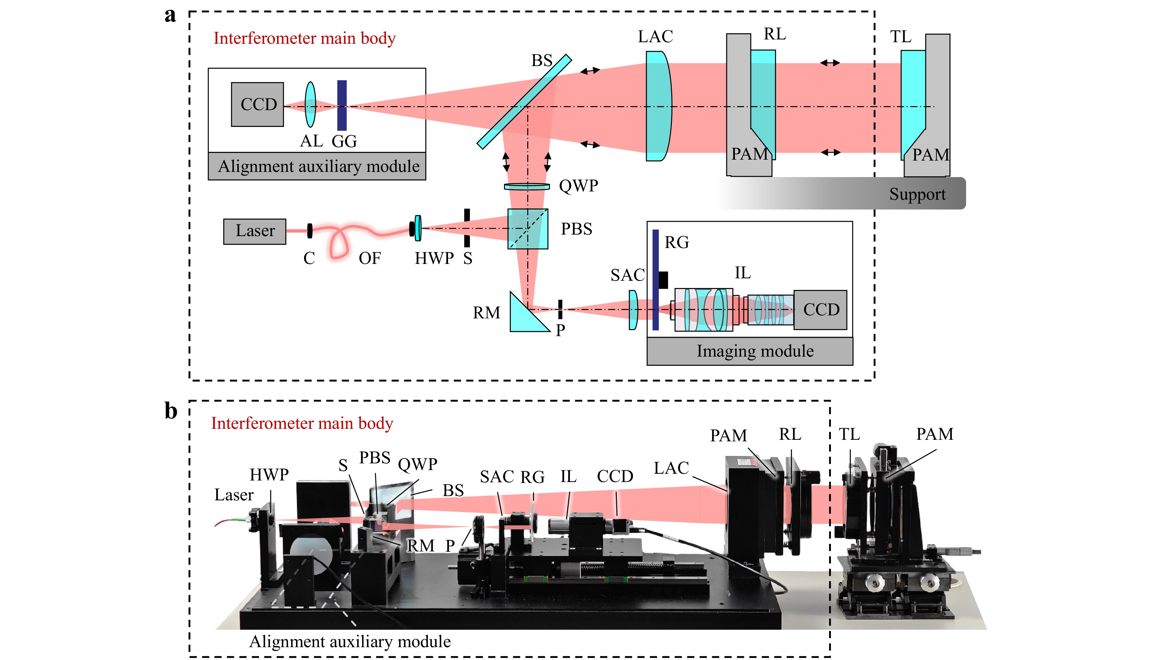
Fig. 5  Optical path diagram a and physical setup b for DII.

We assessed the performance of DII against conventional PSI using a plano-convex lens (effective aperture: 50.8 mm; curvature radius: 64.4 mm). DII experiments were conducted on a standard office desk without vibration isolation, intentionally introducing external vibrations through floor stomping. Conventional PSI experiments, which served as a reference, employed an air-floating vibration isolation platform (AFVI; model ZDT-P-MOT-F, Jiangxi Liansheng Technology Co., Ltd.) and a nanometre high-precision phase shifter (HPPS; model P77.S106, Coremorrow) controlled by piezoelectric ceramics.

The results, illustrated in Fig. 6, demonstrated a strong agreement between DII (Fig. 6b) and conventional PSI (Fig. 6c), with the cross-sectional profiles and surface quality metrics (root mean square, RMS; peak-to-valley, PV) aligned in Fig. 6d. For the spherical surface, DII yielded RMS = 0.0077$ \lambda $ and PV = 0.0511$ \lambda $, which closely matched the conventional PSI values (RMS = 0.0079$ \lambda $ and PV = 0.0554$ \lambda $). For the planar surface, the DII measurements (RMS = 0.6305$ \lambda $, PV = 2.3222$ \lambda $) were closely aligned with the PSI measurements (RMS = 0.6312$ \lambda $, PV = 2.3260$ \lambda $). Differences in the RMS and PV were minimal (order of 0.0001$ \lambda $ and 0.001$ \lambda $, respectively), demonstrating the precision of DII matches that of PSI, despite lacking isolation or a dedicated phase shifter.

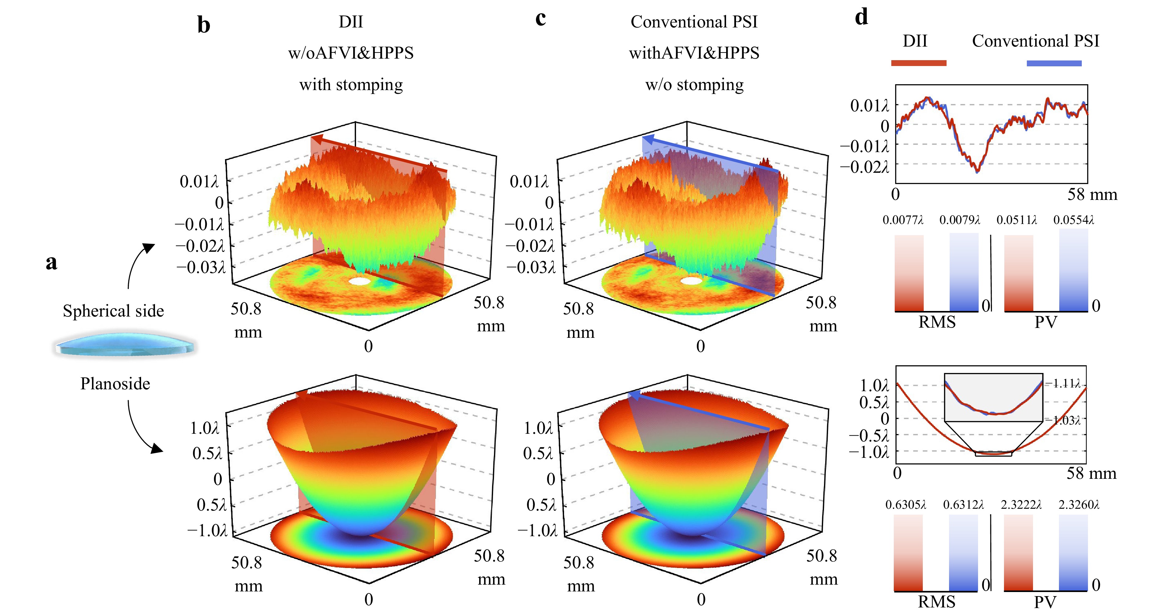
Fig. 6  Comparative measurements of a plano-convex lens. a Test specimen. b DII measurement obtained under induced floor stomping conditions, performed without an air-floating vibration isolation platform (AFVI) or high-precision phase shifter (HPPS). c Conventional PSI measurement acquired using both AFVI and HPPS in the absence of floor stomping. d Comparison of the corresponding surface profiles and associated metrics.

These findings highlight the robustness of DII against vibrations, enabling accurate topographic measurements of optical surfaces under minimal control, and rivalling the performance of PSI under optimised conditions.

Further robustness validation involved measuring the optical flat crystals under various mechanical disturbances under four experimental conditions (C1–C4). Condition C1 utilised a conventional PSI identical to that in the previous experiment, serving as a baseline reference, with PZT actuation as the phase-shifting source (labelled PZT in Fig. 7). Conditions C2–C4 introduced progressively intensified RMD by turning off the air-floating function of the platform (although residual vibration damping remained from the rubber supports). Disturbances for conditions C2–C4 were intentionally introduced via three distinct mechanisms: floor stomping-introduced vibrations (C2, labelled Stmp in Fig. 7), ballscrew-introduced micro-displacements (C3, labelled Scrw), and stress-induced structural deformation of the supporting platform (C4, labelled Defm). While exact replication of these disturbances is challenging, their effects were precisely quantified by differential phase amplitude (DPA), which increased markedly from C1 (0.2326π rad) to C4 (4.3800π rad).

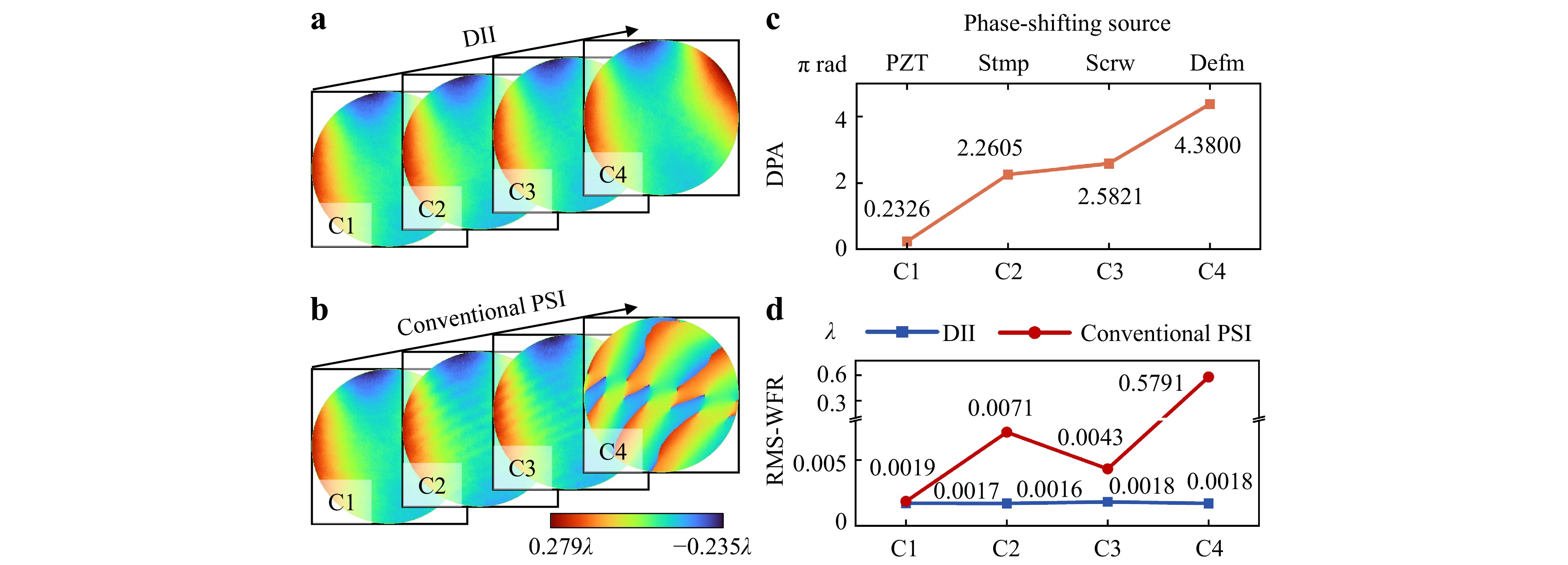
Fig. 7  Surface topography measurements of optical flat crystals under varying conditions. a Surface topography obtained using DII. b Surface topography acquired via conventional PSI. c DPA recorded under different experimental conditions. d Comparison of the RMS wavefront repeatability (RMS-WFR) between DII and conventional PSI across the tested conditions. The phase-shifting sources in C1–C4 are labelled as PZT, Stmp, Scrw, and Defm, corresponding to PZT actuation, floor stomping, ballscrew-introduced micro-displacements, and stress-induced structural deformation of the supporting platform, respectively.

DII demonstrated outstanding consistency across all conditions (Fig. 7a), maintaining stable measurements despite increasing the DPA. In contrast, the conventional PSI measurements (Fig. 7b) significantly deteriorated beyond C1, exhibiting pronounced double-carrier frequency errors under moderate disturbances (C2–C3) and completely erroneous results under extreme disturbances (C4).

Measurement repeatability was quantified via RMS wavefront repeatability (RMS-WFR; defined as the mean RMS difference plus twice the standard deviation for the differential between all even-numbered measurements and a synthetic reference (the average of all odd-numbered measurements; calculation was based on 50 sequential measurements). The measurement repeatability remained stable for DII across all conditions (mean RMS-WFR = 0.0017$ \lambda $), independent of the disturbance intensity. In stark contrast, the RMS-WFR of PSI sharply increased with the disturbance amplitude, peaking at 0.5791$ \lambda $ under C4. This trend was corroborated by additional metrics, as detailed in Supplementary Note 4.

These findings substantiated the effectiveness, precision, and robustness of the DII method under a range of disturbance conditions. For completeness, additional results obtained using a conventional PZT-based configuration without air-floating vibration isolation (AFVI) are provided in Supplementary Note 7. Consequently, we can infer that the DII method is well suited for achieving dependable optical surface topography measurements, even in environments characterised by complex mechanical disturbances.

To address the longstanding reliance on rigorous vibration isolation and phase control inherent in conventional PSI, our paper introduces and demonstrates a method called DII. DII departs from conventional paradigms by reconceptualising random mechanical disturbances as beneficial excitation signals rather than detrimental noise. By leveraging RMDs and employing the NPDA, our method achieves nanometric precision surface-topography measurements without additional hardware.

The robustness of DII is its most significant advantage. Numerical simulations directly comparing the methods under a strong disturbance (DPA = 7π rad) show that DII achieved a remarkable RMSE of just 0.0005λ, whereas conventional four-step PSI completely failed, yielding an RMSE of 0.5λ. Numerical simulations revealed that DII exhibits robustness to nonlinear disturbances over a wide range of DPAs, from 0.01π rad to 12π rad, sustaining a solution success rate above 90% throughout. Experimentally, DII achieved an RMS wavefront repeatability below 0.0018$ \lambda $ in uncontrolled, vibration-prone environments, closely matching the performance of conventional PSI conducted under strictly controlled conditions, with RMS differences as low as 0.0002$ \lambda $ for spherical surfaces and 0.0007$ \lambda $ for planar surfaces.

Regarding the computational cost, the NPDA is built upon well-established numerical techniques, including the CZT for coarse estimation and LM method for iterative refinement, which are efficient and widely used. For a representative dataset of ten interferograms at 512 × 512 pixels, the algorithm was completed in approximately 5 s using MATLAB on a standard laptop computer (12th Gen Intel Core i7-12700H, 16 GB RAM). Using basic code-level optimisations in C++, the processing time was further reduced to less than 1 s. These timescales are within practical requirements of surface metrology applications. Further optimisation remains in practice, and an additional discussion of the computational cost, memory usage, and implementation strategies is provided in Supplementary Note 8. In principle, refinement requires at least three frames. In the simulations reported herein, 10 frames were used as a representative case. However, in practical measurements, a larger number of high-quality frames with sufficient phase diversity is generally preferred for a more reliable reconstruction. Another practical hardware boundary is that the disturbance state should remain approximately constant during exposure to a single camera. Accordingly, the disturbance-induced phase variation within one exposure must remain sufficiently small for each interferogram to be treated as a quasistatic frame. Therefore, the maximum tolerable disturbance frequency depends jointly on the exposure time and disturbance amplitude; otherwise, motion blurring or jelly effect distortions appear.

Despite these promising results, several challenges remain to be addressed. This study focused on mechanical rigid-body disturbances between the test and reference surfaces, which are represented in the current model by frame-dependent piston and tilt terms. In contrast, turbulent airflow introduces phase errors through refractive-index fluctuations in the optical path rather than through rigid-body motion of the optics; therefore, it lies outside the present scope. Its influence on measurement accuracy remains to be investigated in future studies. The applicability range of Eq. (2) should also be noted. The current linear disturbance model is appropriate for planar and low-NA spherical surfaces. For high-NA spherical measurements, additional terms associated with $ \sqrt{1-{\rho }^{2}N{A}^{2}} $ (where $ \rho $ is the normalized coordinate, and NA is the numerical aperture) must be included, requiring corresponding extensions of the model and reconstruction procedure. Moreover, extending the approach to accommodate non-spherical or freeform surface measurements is a compelling direction for future research. In current sub-aperture stitching strategies for non-spherical interferometry, nanometre-scale perturbations between sub-apertures fundamentally limit stitching precision. The adaptive detection capability of DII for such minute disturbances suggests its potential to surmount these limitations. More broadly, the present framework is not inherently restricted to Fizeau geometry. In principle, it can be extended to other PSI-compatible interferometer architectures, such as Twyman-Green and Mach-Zehnder systems, for continuous-wavefront measurements including surface form, wavefront aberration, thickness variation, bow, and warp, provided that an appropriate interferometric forward model is available. However, in its current form, the method is intended for smooth and continuous phase objects. Therefore, it is not directly suitable for rough surfaces, abrupt discontinuities, or complex micro-/nano-structured samples without substantial modifications to both the optical model and the reconstruction algorithm.

Additionally, because the interference model is invariant under simultaneous sign inversion of all phase terms, the NPDA resolves inter-frame sign consistency but cannot determine the absolute orientation of the measured surface (i.e. whether the reconstruction corresponds to +$ \varphi $ or $- \varphi $) from the intensity data alone. In practice, this can be resolved by prior knowledge, such as the known concavity of the test surface or by knowledge of the disturbance direction in at least one frame. This technique also holds considerable promise for integration with common hardware components, such as stepper motors, whose known actuation direction would additionally resolve the absolute sign ambiguity. This would enable more controlled and automated surface topography measurements without the cumbersome hardware characteristics of traditional PSI.

1. In this paper, we propose and demonstrate disturbance-introduced interferometry (DII), in which ambient mechanical disturbances are used as the phase-shifting source, and a natural phase decoding algorithm reconstructs the surface topography from disturbance-modulated interferograms. Numerical and experimental results showed that DII maintains a high measurement accuracy under disturbance conditions, where conventional phase-shifting interferometry degrades severely.

2. The main advantage of the DII is that it reduces the dependence of high-precision interferometric metrology on stringent vibration isolation and precisely controlled phase-shifting hardware. This makes the method particularly attractive for large-aperture optical testing and in situ measurements in vibration-prone manufacturing environments.

3. Future research will extend the present framework beyond the current disturbance model and application scope, including the influence of turbulent airflow, measurement of nonspherical or freeform surfaces, and more general strategies for resolving absolute sign ambiguity.

The authors would like to acknowledge the financial support for this work from the National Natural Science Foundation of China (62375171, 62305208, 62405182, 52127801, 52475563), the Key Research Program of the Chinese Academy of Sciences under Grant RCJJ1452403, the Oceanic Interdisciplinary Program of Shanghai Jiao Tong University (SL2022ZD205), the Science and Technology Commission of Shanghai Municipality (20DZ2220400), Shanghai Innovation Action Plan Project (24ZR1492200), and the Startup Fund for Young Faculty at SJTU (24X010500120).