Analysis and division of full-band errors in optical surfaces

Given the continuous advancement of cutting-edge optical fields such as space optics, extreme ultraviolet (EUV) lithography, and inertial confinement fusion^1–7, stringent requirements have been placed on the full-band errors of their optical components^8–10. Among these, the surface error of optical components (hereafter referred to as a surface error) can be divided into low-, mid-, and high-frequency errors based on their frequency bands. Errors in different frequency bands have distinct and significant effects on the performance of optical systems^11–13, requiring different manufacturing processes for targeted reduction^14–16. Therefore, the accurate division and separation of errors across these frequency bands is an essential requirement in advanced optical manufacturing and testing.

Various standards for frequency-band division have been proposed to facilitate the description and evaluation of surface errors. Initially, standards such as MIL-PRF-13830B¹⁷, ISO 10110 series^18–20, and GB/T 1185-2006²¹ focused on the visibility and dimensions of discrete surface defects rather than serving as standards for error division. Subsequently, institutions such as the U.S. National Ignition Facility (NIF)^22–24 and Zeiss (Oberkochen, Germany)²⁵ have proposed specific error-division standards tailored to their project requirements. However, these standards target optical components for specific tasks, wavelengths, and dimensions. The formulation of some standards relies heavily on empirical rules and lacks a unified and widely applicable standard for frequency-band error division. Consequently, the analysis of frequency-band errors currently relies on manual filtering, which requires multiple adjustments to determine the filtering range. This approach is inefficient, dependent on empirical rules, and prone to introducing operational errors, underscoring the urgent need for a high-precision, high-efficiency, automated, and regularised method for frequency-band error analysis.

In recent years, the field of optical metrology has undergone a methodological shift from traditional numerical computations to machine learning and data-driven paradigms^26–34. To address efficiency limitations, related research has leveraged deep learning to significantly improve feature inference²⁶ and reconstruction speed²⁷, successfully realising the parameter extraction of non-rigid physical models²⁸, rapid mapping of high-dimensional optical responses²⁹, and decoupling analysis of geometric features³⁰. Physics-informed approaches have emerged as a new frontier for overcoming the uninterpretability of pure data-driven models. These methods introduce physical constraints such as energy conservation³¹ and combining simulations with actual measurement data^32–34, thereby enhancing the efficiency and accuracy of complex tasks, including 3D measurement^35–37, phase recovery³⁸, and fringe analysis^39–41. Furthermore, Fourier neural networks and frequency-domain attention mechanisms have recently been integrated into these approaches, demonstrating a significant potential for related tasks such as gradient-based surface reconstruction⁴² and surface defect detection^43,44. However, existing data-driven paradigms have certain limitations:

(1) Traditional methods mostly simplify the problem into black-box image processing, ignoring the physical distribution characteristics of multi-scale information in the frequency domain.

(2) Network training aims to approximate manual labels and can therefore inherit part of the subjective variability introduced by manual filtering if no additional physical constraints are imposed.

(3) Existing solutions frequently rely on high-performance hardware, which makes them difficult to apply in practical engineering sites with limited computational resources.

This study proposes a scale-adaptive physics-aware deep-learning framework driven by a dual-domain physics-aware network (DPN) to effectively mitigate the physical limitations of traditional black-box models and previous fixed-mask methods. Our main contributions are as follows:

1) For the extraction mechanism, the network integrates a deterministic spectral domain selective attention (SDSA) mechanism and a new adaptive learnable spectral gating (LSG) mechanism that targets the distinct spectral distribution characteristics of low-frequency errors and mid-frequency textures.

2) The frequency-domain physical priors help the model to mitigate measurement noise and subjective variability introduced by manual filtering, improving the spectral and physical consistency of the extracted results.

3) We propose a generalised frequency-band division method based on normalised spatial frequency. This framework is designed to achieve the high-precision extraction of full-band errors while targeting millisecond-level real-time inferences on standard computers. The proposed approach can facilitate real-time in situ frequency-band error analysis, providing a foundation for intelligent optical manufacturing and cross-scale cross-instrument optical surface quality evaluation.

The key to accurately extract full-band errors is capturing the physical features of the frequency band errors at different scales from the instrument measurement results. From a traditional spatial domain perspective, the low-frequency surface deviation ($ {Z}_{\text{low}} $), mid-frequency manufacturing texture ($ {Z}_{\text{mid}} $), high-frequency roughness ($ {Z}_{\text{high}} $), and measurement noise ($ N(x,y) $) share the same coordinate space (x,y). Consequently, the distinct frequency-band error features within the instrument testing result ($ Z $) are highly superimposed.

The direct utilisation of neural networks to establish nonlinear mappings in the spatial domain is highly prone to overfitting and lacks physical interpretability because of the vast diversity in the surface morphologies of different optical components. However, according to the Fourier optics theory, superimposed frequency band errors in the spatial domain are naturally separated in the frequency domain⁴⁵, and their spectral amplitudes follow an inverse power-law decay model.

where $ C $, $ k $, and $ \epsilon $ represent a normalisation constant, decay rate constant related to the surface manufacturing process, and minimal value, respectively. This provides a novel perspective for frequency-band error extraction: each frequency-band error exhibits specific information distribution laws in the frequency domain. With an increase in the radial distance $ \sqrt{f_{x}^{2}+f_{y}^{2}} $, the corresponding spatial frequency also increases. Therefore, introducing spectral information distribution as a physical prior into network training is key to enhancing the physical consistency of the extracted results and reducing their sensitivity to local measurement noise and label-dependent fluctuations.

Fig. 1 illustrates the scale-adaptive physics-aware deep learning framework proposed in this study. The framework adheres to the design philosophy of ‘frequency domain awareness and scale adaptation’. An SDSA mechanism is designed based on its isotropic and concentrated spectral information characteristics for the low-frequency error tested by interferometers, and an LSG is designed based on its random and anisotropic spectral information distribution characteristics for the mid-frequency error tested by optical profilers. Both are introduced into the dual-domain neural network as spectral physical information priors for establishing the mapping relationship between the instrument testing results and full-band error. A generalised division of the full-band error is by introducing a normalised spatial frequency to eliminate the size dependence.

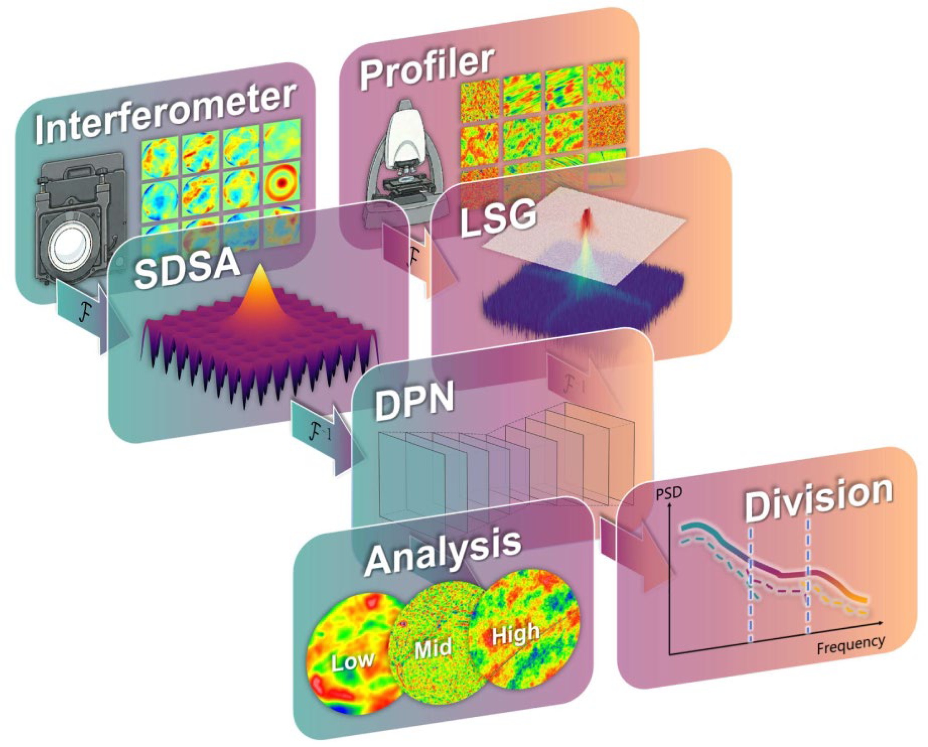
Fig. 1  Scale-adaptive physics-aware deep learning framework. The raw testing results from the interferometer and optical profiler are modulated in the Fourier spectral space by the SDSA mechanism and LSG for low- and mid-frequency errors, respectively. The DPN utilises dual-domain physical constraints to precisely extract the full-band (low-, mid-, and high-frequency) error information from the superimposed raw instrument data, enabling subsequent objective analysis and generalised frequency band error division based on normalised spatial frequency.

Low-frequency errors originate from gravitational deformation, alignment stress, or low-order aberrations⁴⁶, and their spatial domain distribution is continuous and smooth, without obvious directionality. Therefore, the information distribution of the low-frequency error in the frequency domain is fundamentally identical, manifesting as a central envelope with highly concentrated energy and almost no side lobes. Accordingly, we introduce the SDSA mechanism from a previous work⁴⁷ into the DPN, as shown in Fig. 2. The SDSA comprises a spectral attention reinforcer (SAR) and spectral rejection array (SRA).

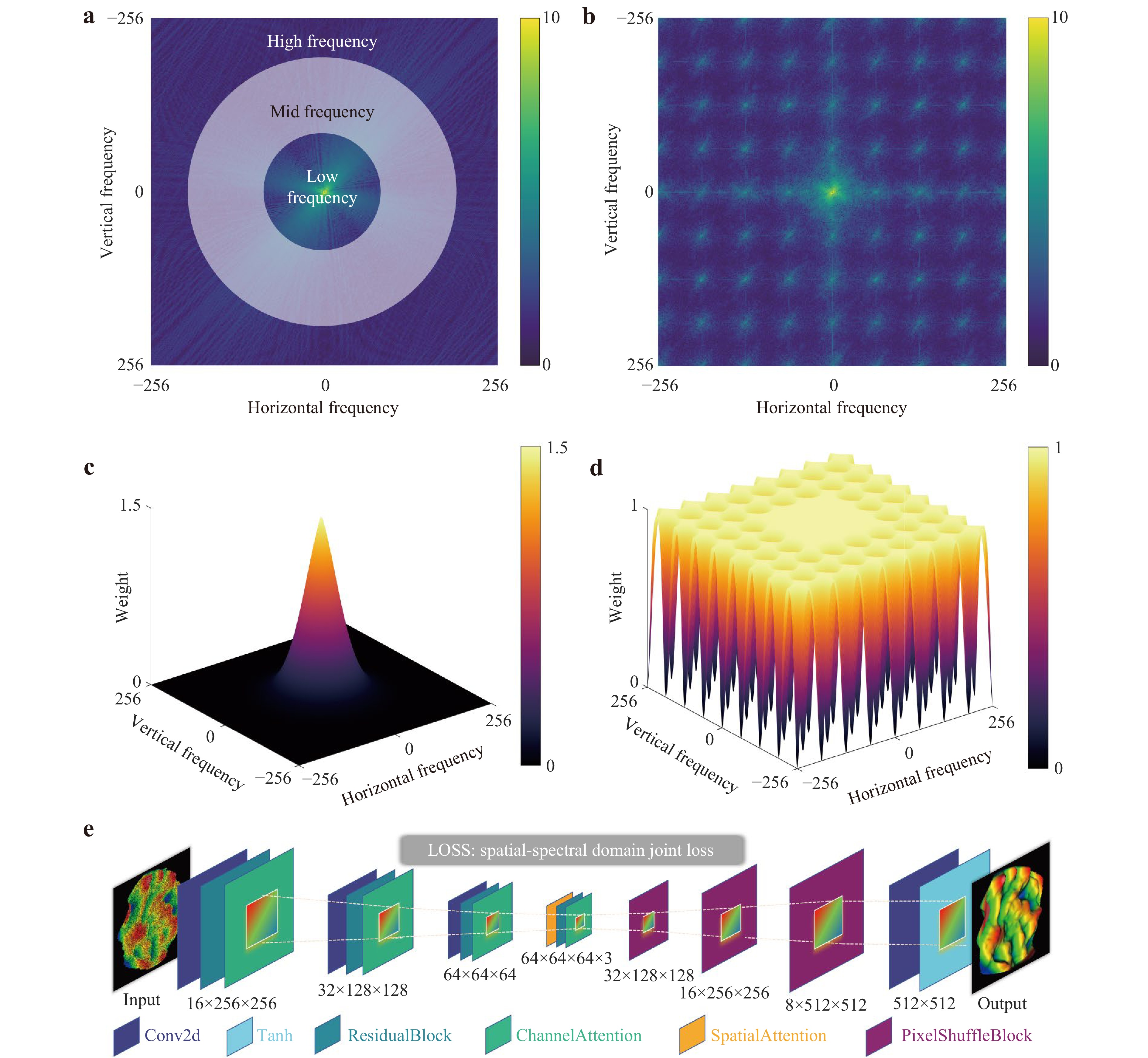
Fig. 2  Architecture of the SDSA and DPN for low-frequency error extraction. a Fourier spectral information distribution characteristics of interferometer testing results, where the frequency gradually increases with the radius. b Distribution of spectral ‘star-like’ noise introduced by traditional convolution during the training process. Based on the above spectra, c and d show the specific designs of the SAR and SRA for low-frequency error, respectively, where SAR is designed as an envelope shape, and the innermost units of the SRA are disabled. e The DPN architecture for low-frequency error extraction.

A detailed theoretical derivation and parameter selection of the SDSA is presented in our previous work⁴⁷. The specific network architecture design is presented in Supplementary Information S2.

Unlike the deterministic spectral envelope morphology of low-frequency errors, mid-frequency errors are primarily introduced during the manufacturing process (e.g. tool marks and vibrations)⁴⁶. The distribution direction and frequency of the mid-frequency errors introduced by the different manufacturing methods are inconsistent, and the spectral information distribution is random with significant anisotropy. Real manufacturing textures are mostly non-ideal sinusoidal morphologies and accompanied by additional vibrations, and therefore, they introduce continuous energy side lobes in the spectrum according to the principles of the Fourier series. Addressing this spectral characteristic, a fixed-morphology mask (such as SDSA) cannot match precisely and easily lead to the loss of valid side-lobe information. Therefore, the extraction of mid-frequency error requires physical constraints that can adaptively fit different spectral morphologies.

To address this challenge, we designed a physics-aware LSG. Unlike the fixed morphology of the SDSA, the LSG adaptively learns the spectral energy distribution of each mid-frequency error. The core mechanism is the introduction of a 3 × 3 frequency-domain convolution kernel to replace traditional point-by-point scanning, which endows the network with a local receptive field in the frequency domain. The LSG is deployed at the front end of the network as a lightweight preprocessing module. Assuming that the input optical profiler testing data is $ Z(x,y) $, it is transformed into the frequency domain $ \widetilde{{Z}_{\rm{in}}}\left({f}_{x},{f}_{y}\right)=\mathcal{F}\left\{Z(x,y)\right\} $ via fast Fourier transform, and its real part $ \text{Re}({\tilde{Z}}_{\rm{in}}) $ and imaginary parts $ \text{Im}({\tilde{Z}}_{\rm{in}}) $ are extracted and concatenated into a two-channel spectral tensor $ {\mathbf{S}}_{\rm{in}}=[\text{Re}({\tilde{Z}}_{\rm{in}}),\text{Im}({\tilde{Z}}_{\rm{in}})] $. This tensor is fed into the LSG subnetwork that is composed of two 3 × 3 convolutional layers and is activated by a sigmoid function to generate a mask ranging from 0 to 1.

where $ \ast $, $ {\boldsymbol{b}}_{2} $, $ \text{BN}(\cdot ) $, $ \text{ReLU}(\cdot ) $, and $ \sigma (\cdot ) $ represent a 2D convolution with a kernel size of 3 × 3, convolutional layer bias, batch normalisation, activation function, and sigmoid function, respectively. $ {\boldsymbol{W}}_{1} $ and $ {\boldsymbol{W}}_{2} $ represent the convolution kernel weights. This convolution kernel design is mathematically equivalent to performing weighted integration within a local neighbourhood of the spectrum, which enables the network to perceive the energy continuity of the surrounding side lobes while evaluating a specific frequency. The generated adaptive mask performs element-wise multiplication ($ \odot $) with the original spectrum to obtain spectral modulation.

Further, it returns to the spatial domain via inverse fast Fourier transform, outputting $ {Z}_{\text{out}}(x,y)={\mathcal{F}}^{-1}\{{\tilde{Z}}_{\text{out}}({f}_{x},{f}_{y})\} $, which is then fed into the backbone network for subsequent extraction. Meanwhile, the DPN backbone adopts an encoder-decoder architecture without skip connections (Fig. 3) to align with the LSG concept, which forces the information to pass through the bottleneck layer for separating the high-frequency random noise and reconstructing the mid-frequency morphology. For specific network construction details and anti-artefact designs, see Supplementary Information S3.

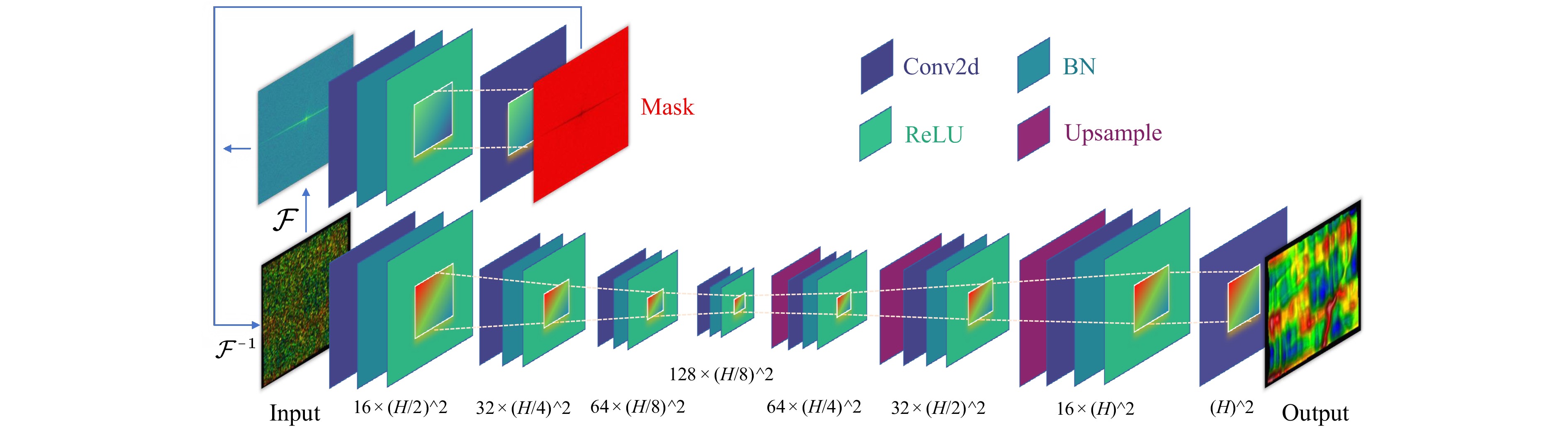
Fig. 3  Design of the LSG sub-network and DPN architecture for mid-frequency error extraction. The front end of the network maps the optical profiler data to the frequency domain through the LSG sub-network (blue line) and generates an adaptive mask to extract mid-frequency topological features. The backbone network adopts an encoder–decoder structure without skip connections, separates additional information through a bottleneck layer, and reconstructs the mid-frequency morphology combining bilinear interpolation for upsampling.

The network training process is driven by a set of multidimensional physical constraint loss functions

where $ {\lambda }_{1} $ and $ {\lambda }_{2} $ represent the hyperparameters used to balance the weights of each loss term. Further, $ {\mathcal{L}}_{\text{spatial}} $ represents the spatial domain mean square error loss, which ensures that the network rapidly learns the overall morphology in the spatial domain, and $ {\mathcal{L}}_{\text{freq}} $ represents the frequency domain amplitude mean square error loss. The spectral energy of optical surfaces spans multiple orders of magnitude, and therefore, direct calculations can cause information in the relatively high-frequency components to be submerged. Therefore, this framework introduces a nonlinear square-root compression to the spectral mean-square error loss.

where $ |\mathcal{F}\{\cdot \}| $, $ {Z}_{\text{gt}} $, and $ \epsilon $ represent the amplitude of the Fourier spectrum, manual label value, and minimal value, respectively. This frequency-domain physical constraint ensures the consistency of the spectral information distribution in the frequency domain. Moreover, mid-frequency textures typically exhibit strong directionality and local gradient mutations. Therefore, the gradient loss $ {\mathcal{L}}_{\text{grad}} $ is introduced to enhance the continuous directional characteristics of the mid-frequency error texture and texture edge details.

where $ \nabla $ represents extraction operators for edge gradients in different directions, implemented in the network using a 3 × 3 discrete difference convolution kernel, and $ \| \cdot \| _{2}^{2} $ represents the L2 norm. Finally, a regularisation term $ {\mathcal{L}}_{\text{mask}} $ based on spectral distance weighting is designed specifically for the LSG mechanism to further suppress high-frequency redundant noise.

where $ \mathbb{E} $ represents the expectation, which calculates the average penalty strength of the mask weights across the entire spectral space. Compared to direct summation, it yields more stable results when dealing with the data of different resolutions, eliminating the need to frequently change hyperparameters. Redundant information and noise in high-frequency regions can be automatically suppressed while preserving valid information in the central area of the spectrum by imposing a weighted penalty based on the radial distance $ \sqrt{f_{x}^{2}+f_{y}^{2}} $. $ {\lambda }_{1}=0.1 $ and $ {\lambda }_{2}=1\times {10}^{-5} $ are the weights. For specific network architecture design, discussions on LSG weight selection, parameter selection experiments, and ablation experiments are provided in Supplementary Information S3.

We constructed two diverse experimental datasets to comprehensively evaluate the full-band error extraction performance of the DPN framework: an interferometer dataset comprising 2,472 samples and an optical profiler dataset comprising 1,853 samples, covering various instrument models, optical apertures, and manufacturing processes. A batch-level isolation strategy was applied during dataset splitting to prevent data leakage (see Supplementary information S4–S6 for details). All baseline models and the proposed DPN were trained and evaluated using the same data split, preprocessing pipeline, manually filtered reference labels, and evaluation metrics to ensure a fair comparison. The hyperparameters were selected according to the validation set performance without providing any model with additional data or label information.

Fig. 4a-c show the DPN performances when processing samples contain typical measurement noise and anomalous bad pixels (spikes). The DPN network not only robustly eliminates anomalous spikes (Fig. 4c) but also extracts a smooth low-frequency error morphology enabled by the spectral physical constraints introduced by the SDSA and sub-pixel upsampling strategy (Fig. 4b). Fig. 4d-h and Table 1 present the quantitative testing results of the DPN on a test set of 371 samples. In terms of precision, the DPN achieves a root-mean-square error (RMSE) of 0.84 nm, which represents a 2.67-fold improvement in accuracy compared to that of the baseline CNN. The relative accuracy (Rel Acc) is introduced to clearly evaluate the similarity between the extracted error and manual labels, defined as

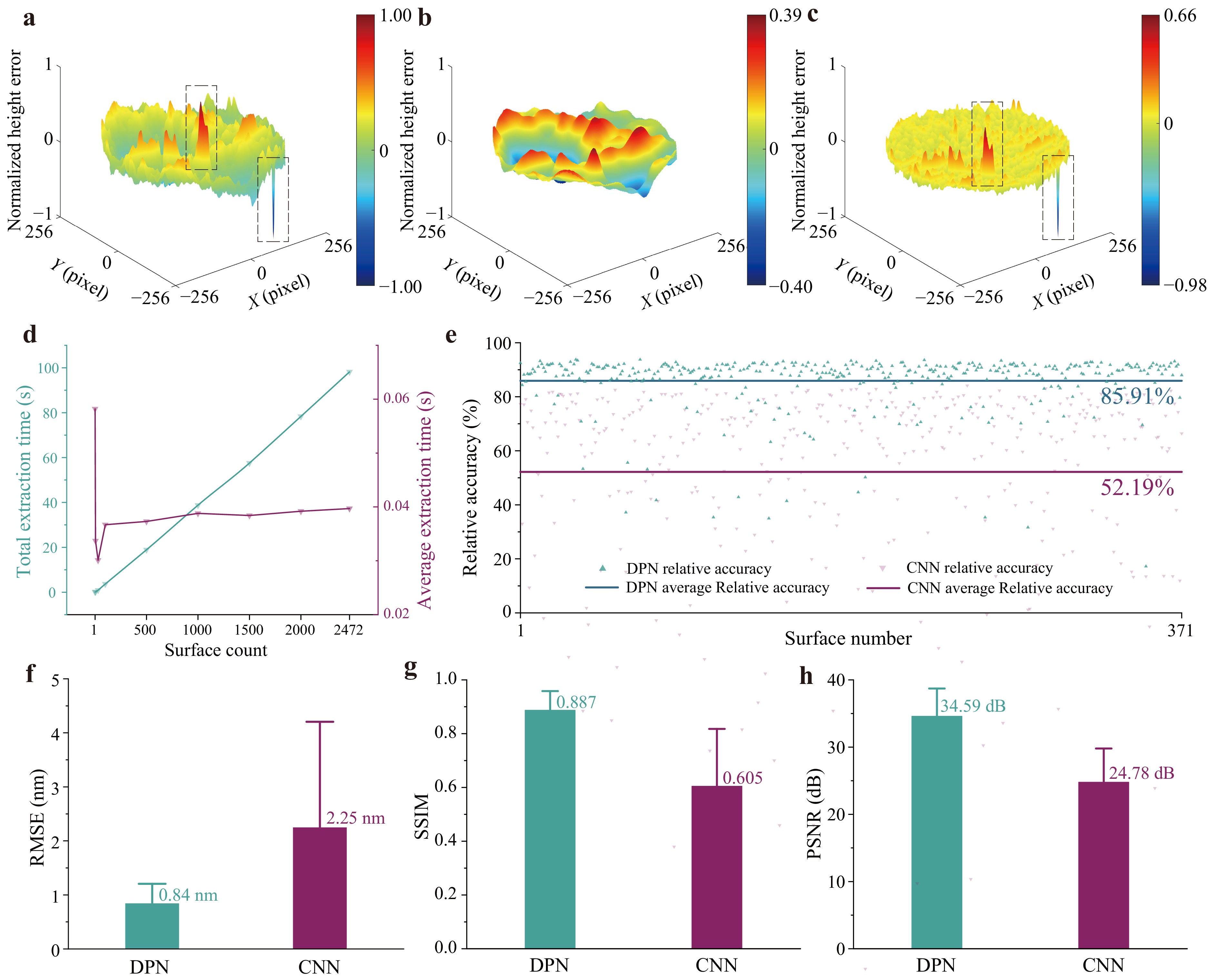
Fig. 4  Performance demonstration of the DPN for low-frequency error extraction. a-c Demonstration of outlier elimination: a Raw interferometer input containing anomalous spikes. b Smooth low-frequency error extracted by the DPN. c Residual map between the two, which shows that two anomalous spikes are effectively removed by the DPN. d Total extraction time and average extraction time per surface for different inputs by the DPN. e-h Quantitative comparison between the DPN and baseline CNN on four core evaluation metrics: relative accuracy, RMSE, SSIM, and PSNR.

where $ {{RMS}}_{\text{gt}} $ represents the root mean square of the manual label. Across key metrics such as relative accuracy (85.91%), structural similarity (SSIM, 0.887), and peak signal-to-noise ratio (PSNR, 34.59 dB), the DPN consistently outperforms the comprehensive baseline set, which includes the classic spatial-domain (U-Net, Transformer, PINNs) and advanced frequency-domain architectures (physics-informed FNO (PI-FNO) and U-Net-based adaptive FNO (U-AFNO)) as demonstrated in the updated Table 1. In terms of computational efficiency, as shown in Fig. 4d, the DPN requires an average of only 0.04 s to process a single surface error map on a standard laptop without GPU acceleration (see Supplementary Information S2 for details), which is an improvement of nearly 750 times compared to that of traditional manual filtering (~30 s/surface).

Fig. 5 shows the adaptive perception mechanism of the LSG for different spectral morphologies. For surfaces with different roughness values (Fig. 5a), the spectral energy distributions exhibit distinctly different morphologies (Fig. 5b). The LSG effectively generates corresponding masks dynamically for different spectra (Fig. 5c), precisely identifying the valid information regions. The effect of the convolution kernel scale on topological perception, the parameter selection experiments in Supplementary information S3 indicate that the LSG effectively addresses the limitation of traditional 1 × 1 point-by-point filtering owing to the local receptive field introduced by the 3 × 3 convolution kernel, which tends to truncate weak side lobes. It can dynamically generate continuous masks that cover the complete key information regions of the different spectra. This mechanism ensures the complete recognition of the network of mid-frequency features while continuously suppressing redundant noise in high-frequency regions.

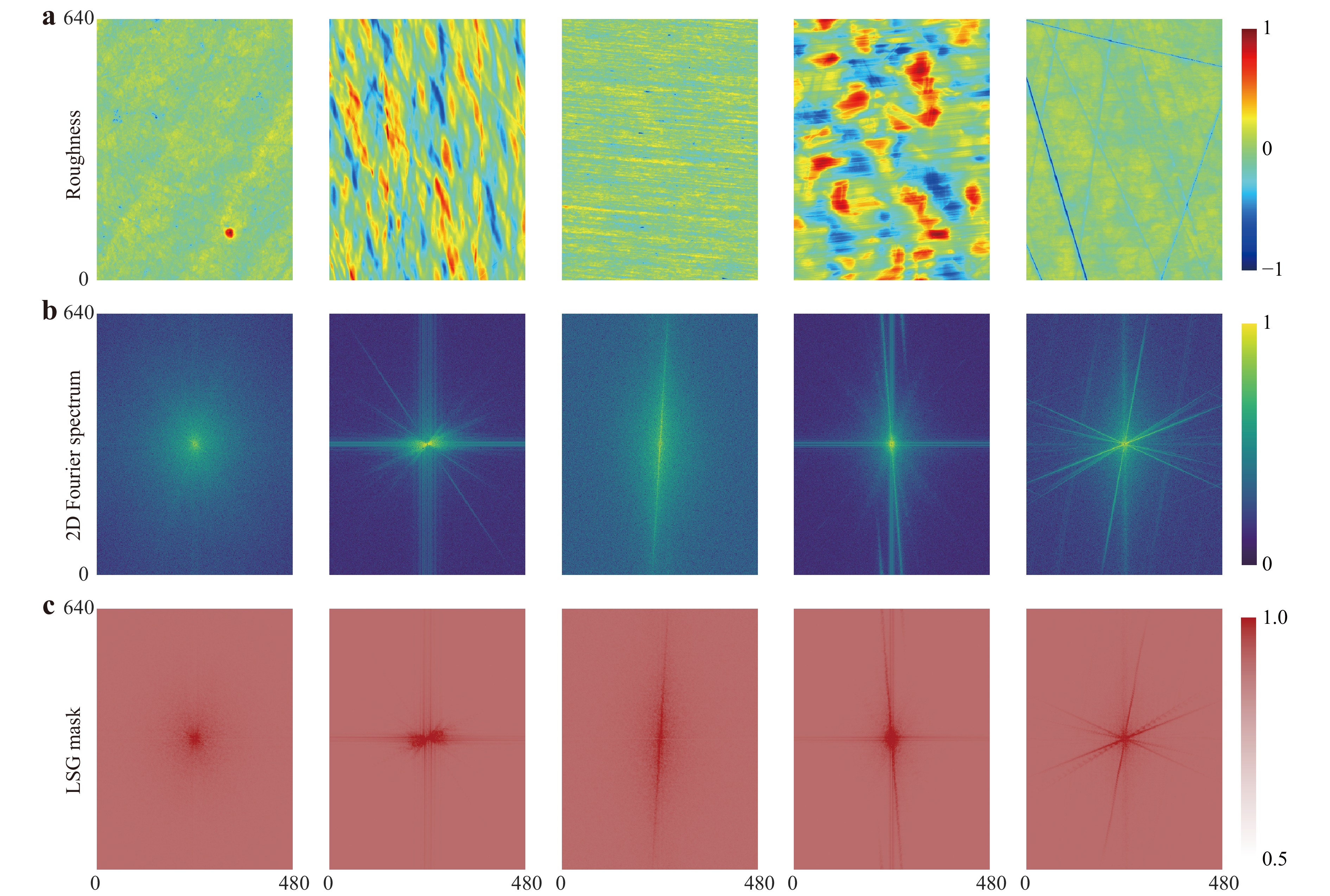
Fig. 5  Adaptive perception effect of the LSG on different mid-frequency morphologies. a Raw optical profiler testing results of five groups with typical manufacturing textures. b Corresponding five 2D Fourier spectra, which present anisotropic energy distribution characteristics. c Frequency domain mask generated by the LSG based on spectral features, achieving the precise coverage of the key information distribution regions.

Based on 279 test samples, Fig. 6 and Table 2 present the qualitative and quantitative extraction performance of the DPN for the mid-frequency error. The high-frequency roughness can be separated simultaneously and in real time from the raw data using a simple subtraction operation because the optical profiler testing data are essentially a superposition of mid- and high-frequency errors enabled by the high-precision decoupling of the DPN of the mid-frequency error(Fig. 6d, e). In terms of accuracy metrics, the DPN achieved an RMSE of 0.37 nm and a relative accuracy of 86.29%, which consistently outperforms the comprehensive baseline set, including classic spatial-domain architectures (U-Net, PINNs, and Transformer) and advanced Fourier-domain architectures (PI-FNO and U-AFNO) across key metrics such as SSIM (0.905) and PSNR (36.02 dB), as demonstrated in the updated Table 2. In terms of computational efficiency, the DPN requires an average of only 0.05 s to process a surface error map, which is an improvement of nearly 600 times compared to that of traditional manual filtering (~30 s/surface).

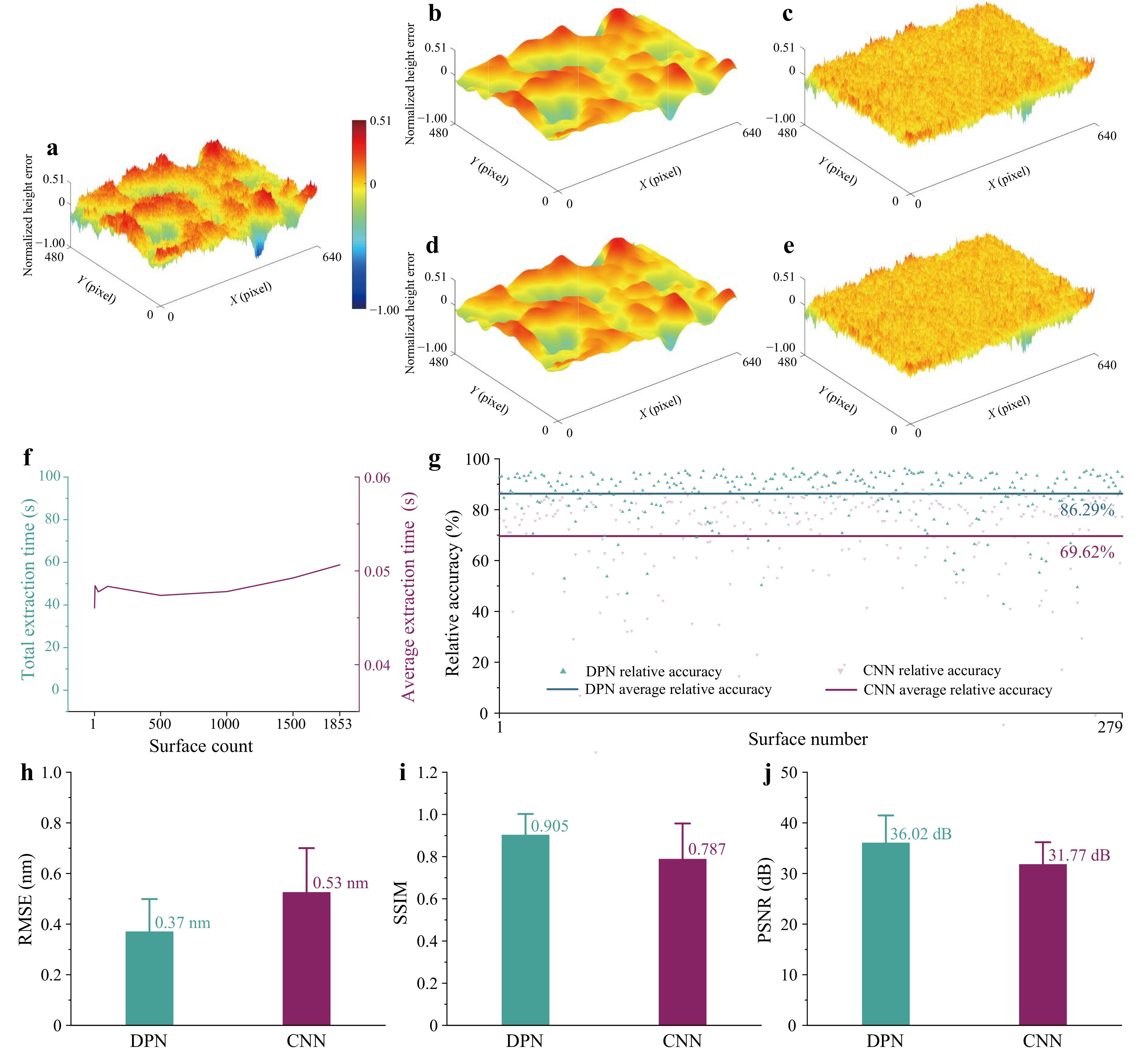
Fig. 6  Performance demonstration of the DPN for mid-frequency error extraction. a Raw optical profiler testing input. b and c Manually filtered references for the mid- and high-frequency errors. d and e Extraction results of the DPN for the mid- and high-frequency errors, respectively. f Total extraction time and average extraction time of the network for different inputs. g-j Comparison between the DPN and baseline CNN on relative accuracy, RMSE, SSIM, and PSNR.

The performance of traditional data-driven methods are constrained by the subjective noise of manual labels, which inherently risks propagating subtle biases in the outputs of the model. However, the DPN mitigates this problem by learning physical commonalities from large-scale datasets to statistically smooth out individual randomness. In the aforementioned quantitative evaluation, the DPN achieved high accuracy in the RMSE; however, the SSIM and relative accuracy did not yield perfect matches. This phenomenon reveals the distinct ‘physics-correction effect’ of the DPN. This effect refers to an observed output behaviour rather than an independent label-free correction module: under the basic supervision of manually filtered references, frequency-domain physical priors, dual-domain constraints, network architecture, and training regularisation jointly reduce the mechanical fitting of the model to local label anomalies and subjective filtering variability, producing results with improved spectral and physical consistency. The contributions of the main physical constraints and network settings are supported by the ablation study presented in Supplementary information S3.2.

In the extraction of low-frequency error, the ‘physics-correction effect’ manifests as the suppression of outliers. As shown in Fig. 7a-c, the DPN does not mechanically fit the anomalous spike noise introduced during the instrument testing process; however, it outputs a smooth and continuous low-frequency error. The quantitative power spectral density (PSD) curves (Fig. 7g, h) more clearly support this effect. The extraction results of the DPN show better consistency with the expected low-frequency spectral distribution across the full band, which suggests that the network can suppress local measurement defects in the manual reference rather than simply replicating them. In the extraction of a mid-frequency error, the ‘physics-correction effect’ is even more pronounced. A conservative filtering strategy is usually adopted because manual filtering struggles to precisely determine the cutoff frequency; This leads to the loss of a large amount of small-scale tool mark information (Fig. 7d, e). Conversely, the DPN is less affected by the conservatism of manual labels and preserves more mid-frequency texture components under spectral constraints (Fig. 7f). The PSD curve in Fig. 7i quantitatively shows that the DPN maintains stronger spectral components than the conservative manual reference within the critical frequency band of 10¹–10² mm^–1. The DPN is not a simple label-fitting model. By leveraging the statistical advantages of large-scale data combined with dual-domain physical constraints, this approach mitigates the subjective randomness of manual operations and provides a method for full-band error feature extraction in practical engineering applications.

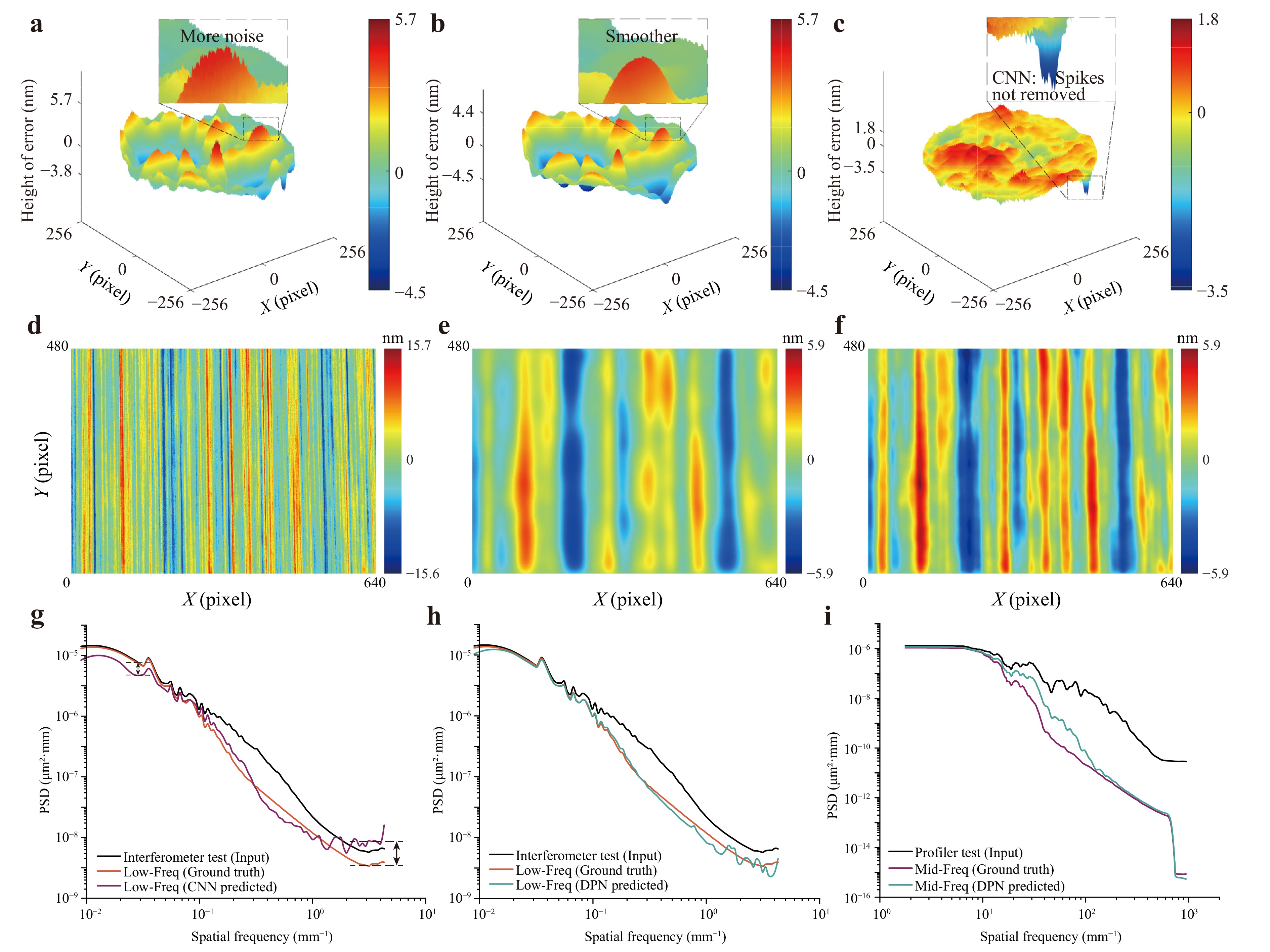
Fig. 7  ‘Physics-correction effect’ of the neural network and its quantitative PSD analysis. a-c Comparison of low-frequency error: a CNN extraction result containing anomalous spikes, b Smoother and continuous DPN extraction result. c Residual map between the two, showing that the DPN can suppress anomalous spikes and high-frequency noise. d-f Comparison of mid-frequency error: d Raw input containing dense periodic fluctuations. e Manual reference loses details caused by conservative filtering. f DPN extraction result preserving more small-scale textures. g-i Corresponding quantitative PSD analysis, which shows that the DPN retains more spectral features in the low-frequency band (g, h, spatial frequency < 10⁻¹ mm⁻¹) and the critical mid-frequency band (i, 10¹ < spatial frequency < 10² mm⁻¹), while avoiding the introduction of additional high-frequency noise.

The division of frequency-band errors is a bridge connecting optical manufacturing and testing. Existing division standards (such as ISO 10110 and MIL-PRF) are often based on fixed spatial frequency thresholds (e.g., 1 mm⁻¹), which results in the same physical frequency having entirely different physical meanings for components of different sizes or under different testing fields of view, thereby lacking generalisability. To address this issue and based on the objective features of frequency band errors learned by the DPN on massive data, we propose a generalised division method based on the normalised spatial frequency. The normalised spatial frequency is defined as

where L represents the instrument testing aperture of the current data. In contrast to the full aperture D of the optical component, selecting L holds stricter physical significance: mid- and high-frequency textures are determined by the manufacturing process and have no direct correlation with the full aperture D of the optical component. Normalisation based on L not only avoids the distortion of evaluation standards caused by excessively large spans in component sizes but also better aligns with human visual perception, realising a dimensionless cross-scale and cross-instrument evaluation with the fluctuation period of the current field of view as the dimension.

When determining the specific division boundaries, we calculated the average PSD curves of the raw testing data and the DPN extraction results, and we introduced a ‘variance index’ to quantify the degree of separation between the two to objectively define the critical point. As shown in Fig. 8, the frequency-band breakpoints for interferometer or optical profiler data converge at a normalised spatial frequency of 8. To balance the signal-to-noise ratio, the breakpoint of 7.2 from the previous work⁴⁷ was optimised under the current data, which indicates that, within any testing field of view, a fluctuation period greater than 1/8 of the field of view is classified as low frequency, and less than 1/8 is classified as high frequency. This value provides an engineering division point for the datasets and testing conditions considered in this study, effectively reducing the subjective randomness induced by manual empirical rules. The normalised spatial frequency framework provides a general method by which users can determine suitable frequency band boundaries according to their instruments, component sizes, and engineering requirements. This breakpoint should be understood within the scope of the present engineering datasets rather than as a mandatory cross-institutional standard because independent multi-institutional datasets are yet to be included.

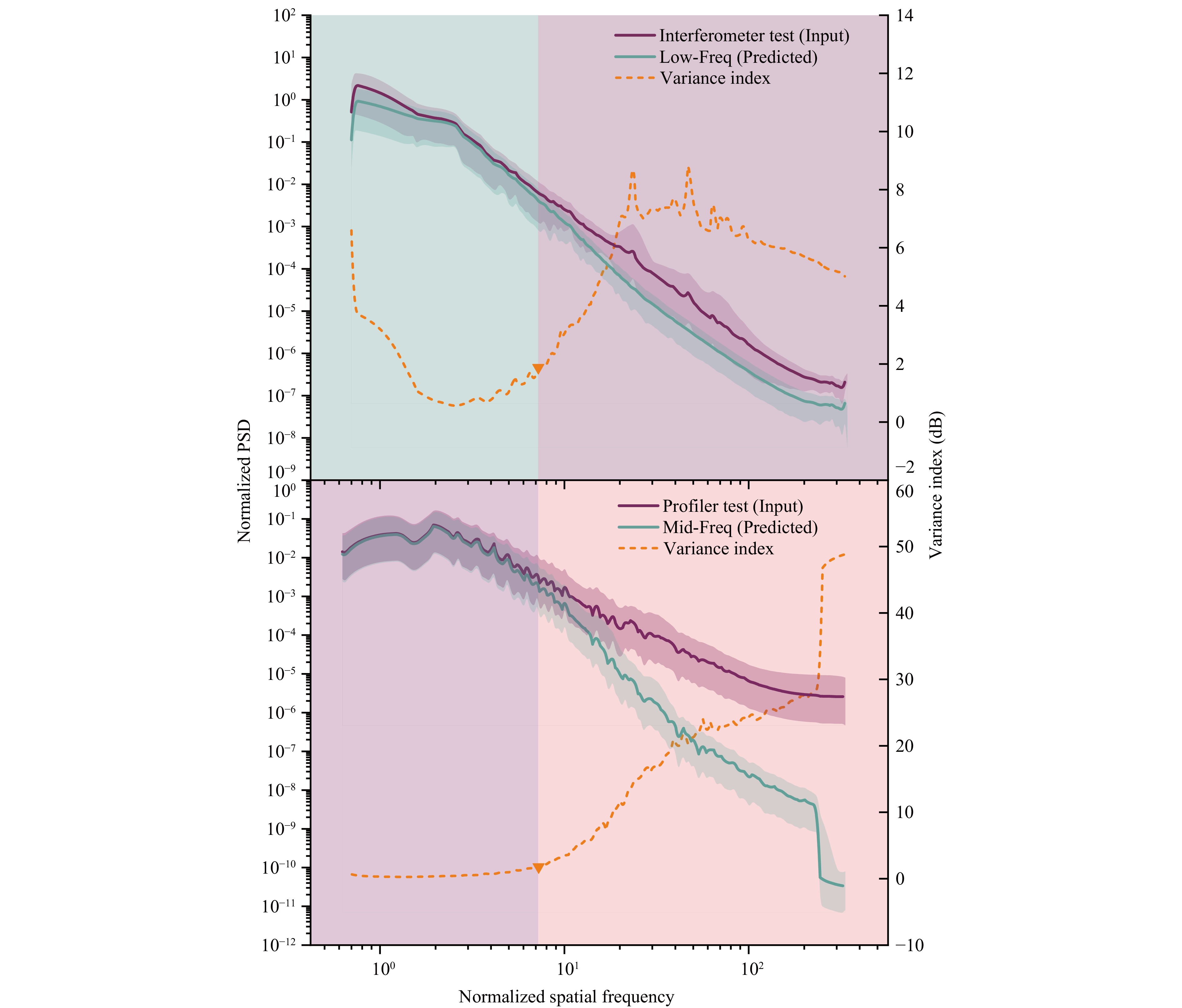
Fig. 8  Generalised division of full-band errors based on normalised spatial frequency. The upper and lower panels show the average PSD curves of the testing data and their DPN extraction results for the interferometer (low frequency) and optical profiler (mid frequency), respectively. The light shaded bands represent the standard deviation of the datasets. The variance index quantifies the degree of separation between the extraction results and raw instrument testing data. The variance index exhibits an upward trend in the frequency band error transition zone because of the coupling between frequency band errors. For the boundaries between low- and mid-frequency errors, as well as between mid- and high-frequency errors, the breakpoints are both at a normalised spatial frequency of 8.

This study proposed a physics-aware dual-domain deep learning framework driven by a DPN to effectively address the bottlenecks of low efficiency, strong subjectivity, and inconsistent frequency-band division criteria in cross-scale optical surface testing. The DPN addresses the mechanical fitting of manual labels inherent in traditional black-box models by integrating the spectral features as explicit physical priors into the network design (SDSA and LSG). On a standard computer, this framework achieves high-precision extraction of full-band errors with a millisecond-level (0.05 s) inference efficiency, outperforming existing data-driven methods and establishing the advantage of physical priors in solving complex optical metrology problems.

The contribution of this study lies in demonstrating a physics-constrained extraction framework for full-band surface errors, and based on this, it is to refine the evaluation strategy. Relying on dual-domain constraints and statistical laws, the DPN mitigates measurement noise and subjective variability inherent in manual filtering, producing extracted results with improved spectral and physical consistency. Based on this, we established a generalised frequency band division method based on normalised spatial frequency. This method not only possesses crossband transfer learning capabilities but also addresses the challenges of size dependence in multi-instrument collaborative testing by providing a normalised-frequency-based workflow for frequency-band error division. Moreover, the applicability of the DPN is not inherently limited to specific aperture shapes or base geometries as a generalised physical-feature-aware architecture. Further, the framework demonstrates a promising potential for generalisation to complex surfaces. However, the DPN may deviate from the optimal reconstruction owing to overlapping physical features or sampling distortion under extreme conditions such as highly aliased complex periodic textures (see Supplementary Information S10). Owing to the current scarcity of open-source optical surface datasets, future work will focus on cross-validating the framework using multi-institutional data. The diagnostic scope of the DPN framework can be extended in future studies to include the quantification of localised surface defects and scatterers, providing a more comprehensive toolset for automated surface inspection.

This paradigm provides a practical engineering solution by translating data-driven metrics into downstream optical-performance gains. For the wavefront quality, the high-fidelity low-frequency errors extracted by the DPN provided a reliable baseline for deterministic polishing, effectively removing measurement noise crosstalk (see Supplementary Information S9). Moreover, through the precise decoupling of roughness data, the DPN simultaneously isolates high-frequency errors to evaluate scatter reduction for high-end systems, such as EUV optics, while preserving mid-frequency tool marks to trace the machining status and improve manufacturability. Finally, achieving millisecond-level inferences with low hardware reliance yields process-control benefits. This propels existing optical testing from ‘offline empirical analysis’ to ‘real-time in situ closed-loop feedback’, laying a solid foundation for automated optical manufacturing.

This work was supported by the National Major Research Instrument Development Project (62127901), Independent Project Task Document of the Key Laboratory of Advanced Manufacturing of Optical Systems (Chinese Academy of Sciences) (KLMSZZ202305), and Research on the Key Technology of Rapid Synchronous Detection of Surface Shape and Subsurface Defects in the Grinding Stage of Large-Diameter complex surface (2025010157).