


-
One of the most important aspects of a modern product is its surfaces; both shape and fine-scale topography are critical when considering tolerances, assembly, and, ultimately, functionality1. Surfaces are highly sensitive to changes in the manufacturing process and can be diverse and complex, owing to various functional specifications and the characteristics of the manufacturing processes.
In tribology, surface interactions influence the friction, wear, and lifetime of a component. It is estimated that surface effects cause 10% of manufactured parts to fail, which can have a significant repercussion on a country’s GDP1. In fluid dynamics, surfaces determine how fluids flow; in aircraft, for example, this affects aerodynamic lift and thereby influences fuel consumption. Biomimetic surfaces can be engineered to significantly affect functions such as hydrophobicity, colour, and hardness2. Structured surfaces apply to food-packaging applications3, and interest has risen recently in how COVID-19 adheres to different surfaces4.
In 2019, the first international specification standard was published, which goes some way towards establishing a framework for calibrating areal surface-topography measuring instruments, including those employing optical techniques5. The path to the development of ISO 25178 part 600 is summarised elsewhere6–8 and was recently reviewed9. This paper will present a different, although complementary, approach to measurement uncertainty, based on developing an accurate physical model of the measurement process.
One approach to uncertainty evaluation, common in the coordinate metrology world, is to use a “virtual instrument”. A virtual measurement system considers the various influence factors and simulates the measurement using an accurate model that mimics the real measurement process. The influence factors can be varied, based on appropriate stochastic models, and a large number of simulated measurements can be generated to evaluate the combined measurement uncertainty. For objects with complex geometries, virtual coordinate-measurement machines10-13 are often the only means to evaluate task-specific uncertainty for contact instruments. The technique is outlined in ISO/TS 15530 part 414 and has been adopted by industry, using commercially available software.
There has been limited development of virtual instruments for contact-stylus surface measurement15,16; but however, virtual instruments are not yet available in the context of optical surface metrology because of the complexity of optical measurement and the large variety of surface types. The closest technique to a virtual optical instrument is the method proposed in reference 17, which simulates the measurement error of a surface-measuring microscope, based on an empirical Gaussian process model. This method has been used for task-specific uncertainty evaluation in focus-variation microscopy for several case studies.
However, this method neither directly models physical phenomena, e.g. surface scattering and three-dimensional (3D) image formation with a finite numerical aperture (NA), nor captures systematic errors. Similar to virtual coordinate-measurement machines, the direct output of the simulator is a point cloud, not (3D) image data. It is worth noting that in all optical surface-measuring techniques, the surface topography is reconstructed from the 2D/3D image data (or 1D optical signal for point-measurement techniques). The surface-reconstruction algorithms are varied and can introduce additional errors. Therefore, it is important to separate the image-formation and surface-reconstruction processes in a virtual optical instrument, in the same manner as in a real instrument.
The modelling of optical surface-topography measurements has advanced considerably, providing details of the interaction of light with complex surface structures18, multiple scattering19, the effect of dissimilar materials20,21, semi-transparent surface films20,22, and optically unresolved structures23. There are also many examples of instrument modelling for specific sources of measurement error, e.g. camera noise24,25, environmental vibration26, and optical aberrations27,28. Instrument models have been developed to solve inverse problems that rely on simulating signals for comparison with experimental results23,29. Nonetheless, from the perspective of the instrument user in industry, the development of virtual optical instruments remains a critical but unmet need.
In this paper, we will present the development of a physics-based virtual optical instrument for surface measurement, specifically a virtual coherence scanning interferometer (CSI), where coherence scanning interferometry is a well-established, widely used technique for areal surface measurement30-32. The primary function of the virtual instrument is task-specific uncertainty evaluation; it can also be used to predict instrument responses and measurement results, in order to assess the feasibility of an instrument for a specific surface, find optimal instrument settings, improve the understanding of the measurement process, and test new instrument configurations. The scope of this paper will be limited to the concept, theory, development, validation, and demonstration of the proposed virtual CSI. The software to implement the virtual CSI will be made publicly available. Task-specific uncertainty evaluations will be presented in future work.
-
A physics-based virtual CSI is effectively a “digital twin” of a real CSI (Fig. 1). The virtual instrument considers all the major influence factors and simulates surface measurements using a combination of physical models, with calibrations based on an actual target instrument. A key component is an appropriate 3D imaging model. In this work, we consider the linear theory of coherence scanning interferometry, based on a foil model of the surface33.
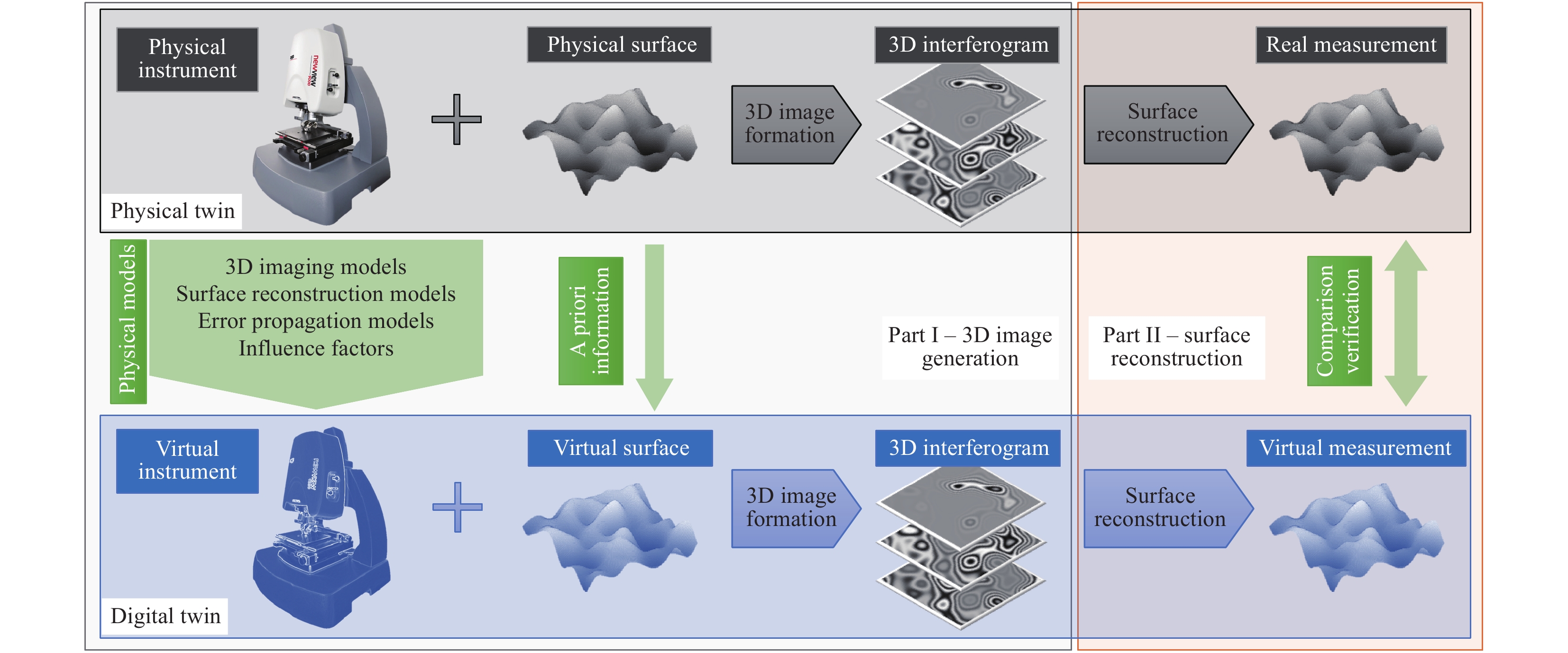
Fig. 1 Concept of the virtual CSI.
Surface parameters can be evaluated based on the virtual-measurement result (Interferometer image courtesy of Zygo Corporation).In this theory, the conditions for the validity of the Kirchhoff approximation for surface scattering must be satisfied, and 3D interferogram generation is expected to be a linear-filtering process applied to the foil model of the surface. The linear-filtering process is characterised by a 3D surface-transfer function (STF). It has been shown elsewhere that 3D image formation in a CSI can be calculated from any appropriate surface-scattering model34, including numerical techniques to solve Maxwell’s equations exactly19.
Thus, the proposed method can be extended to the nonlinear regime, where multiple scattering, dissimilar materials, transparent films, and polarisation effects are considered. Appropriate error-generation models are used to incorporate the effects of various influence factors into the 3D interferogram of a CSI. The influence factors can be varied, based on their known values or as probability distributions, as part of an uncertainty evaluation.
A priori knowledge about the surface, e.g. the as-designed surface model or a reference measurement provided by a traceable instrument, is used as the “true” surface to initiate the virtual measurement. Defining a true surface through simulation is an advantage of the virtual-instrument approach for measurement-error prediction, as opposed to empirical measurements with material measures. A direct comparison between the true and virtually measured surfaces leads to a position-dependent measurement error map for parts having a comparable structure, without uncertainty contributions from the reference measurement used to certify the material measures.
-
We first introduce the underpinning theory of the virtual CSI, and then describe the instrument setup on which the virtual-CSI development is based. The major influence factors of a virtual surface measurement are indicated, along with the instrument configuration. This is followed by an illustration of the virtual measurement process and how the influence factors are applied. Finally, the models for incorporating vibration, actuator linearity, camera noise and camera bit depth, lateral distortion, and flatness into the virtual measurement are described.
-
The proposed virtual CSI is underpinned by the linear theory of coherence scanning interferometry for surface measurement, based on a foil model of the surface. We will briefly introduce the theory; a detailed derivation can be found elsewhere33,34. In a CSI, the surface topography is derived from a camera-recorded 3D interferogram, which is given by
$$ I\left({\bf{r}}\right)=2{\rm{Re}}\left\{O\left({\bf{r}}\right)\right\} $$ (1) The complex-valued interferogram term
$ O\left({\bf{r}}\right) $ can be considered as a convolution of the foil model of the surface$ F\left({\bf{r}}\right) $ and the shift-invariant 3D point-spread function (PSF)$ H\left({\bf{r}}\right) $ , as$$ O\left({\bf{r}}\right)=F\left({\bf{r}}\right)\otimes H\left({\bf{r}}\right)$$ (2) where
$ {\bf{r}}={r}_{\rm{x}}\widehat{\bf{x}}+{r}_{\rm{y}}\widehat{\bf{y}}+{r}_{\rm{z}}\widehat{\bf{z}} $ in a Cartesian coordinate system. The foil model is expressed as33$$ F\left({\bf{r}}\right)=RW\left({\bf{r}}\right)\delta \left[{r}_{z}-{Z}_{s}\left({r}_{x},{r}_{y}\right)\right] $$ (3) where
$ \delta \left(\right) $ is a 1D Dirac delta function that follows the surface height,$ {Z}_{s}\left({r}_{x},{r}_{y}\right) $ , of a homogeneous material as a function of the lateral position,$ R $ is the amplitude reflection coefficient, and$ W\left({\bf{r}}\right) $ is an appropriate shading function33,34. For a perfect conductor, the reflection coefficient$ R=1 $ . More generally,$ R $ is approximately constant for angles of incidence that are less than 45°33,34.In the spatial-frequency domain (
$ {\bf{K}} $ -space, where$ {\bf{K}}={K}_{\rm{x}}\widehat{\bf{x}}+{K}_{\rm{y}}\widehat{\bf{y}}+{K}_{\rm{z}}\widehat{\bf{z}} $ ), the spectrum of the 3D interferogram can be considered as a filtered version of the foil model,$$ \tilde O\left({\bf{K}}\right)=\tilde F\left({\bf{K}}\right)\tilde H \left({\bf{K}}\right) $$ (4) The filter
$ \tilde H \left({\bf{K}}\right) $ is called the 3D STF, and the Fourier transform of the 3D STF gives the 3D PSF. The 3D STF is generally complex-valued; its magnitude weights the Fourier components of the surface’s foil model and characterises the passband of the instrument. Its phase is related to optical aberrations of the instrument (the phase term will be zero if the instrument is diffraction-limited). For a CSI with an extended broadband source and a fully filled illumination pupil, the 3D STF is expressed as34$$ \tilde H \left({\bf{K}}\right)=\frac{{{\bf{K}}}^{2}}{16{{\text{π}} }^{3}{K}_{z}}\int \int {\tilde G }_{NA}\left({\bf{K}}-{\bf{K}}',{k}_{0}\right){\tilde G }_{NA}\left({\bf{K}}',{k}_{0}\right){d}^{3}{K}^{'}\frac{S\left({k}_{0}\right)}{{k}_{0}}d{k}_{0} $$ (5) where
$ {k}_{0}=2{\text{π}} /\lambda $ is the wavenumber. The broadband source, e.g. a white-light light-emitting diode (LED), is characterised by a normalised power-spectrum density$ S\left({k}_{0}\right) $ . The generalised 3D pupil function35, subject to a finite NA (denoted by$ {A}_{N} $ ), is a spherical shell in the wave-vector (k) space and can be expressed as34$$ {\tilde G }_{NA}\left({\bf{k}}\right)=\frac{2{{\text{π}} }^{2}}{{k}_{0}}\delta \left(\left|{\bf{k}}\right|-{k}_{0}\right){H}_{step}\left({\bf{k}}\cdot \widehat{\bf{z}}-{k}_{0}\sqrt{1-{A}_{N}^{2}}\right)A\left({\bf{k}}\right) $$ (6) where
$ {H}_{step}\left(\right) $ is the Heaviside unit step function. The pupil apodisation function$ A\left({\bf{k}}\right)=1 $ corresponds to a uniform angular apodisation (the Herschel condition), and$ A\left({\bf{k}}\right)=\sqrt{{\bf{k}}\cdot \widehat{\bf{z}}/{k}_{0}} $ corresponds to a perfect aplanatic case34,36. The illumination pupil can also be apodised and characterised by a suitable distribution function. For example, in the case of a Mirau objective, the central obscuration by the reference mirror will influence the apodisation of both the illumination and observation pupils.The major limitation of the linear theory of coherence scanning interferometry is the validity regime of the Kirchhoff approximation for surface scattering34,37. The major condition for validity is that the radius of curvature at any surface point is much larger than the wavelength. Here, we consider the criterion proposed by Brekhovskikh (see Section 3.3 in ref.37),
$$ {C}_{R}=\frac{4{\text{π}} {r}_{c}{\rm{cos}}\theta }{\lambda }\gg 1 $$ (7) where
$ {r}_{c} $ is the radius of curvature at a surface point and$ \theta $ is the local angle of incidence. Therefore, the surface must not contain sharp edges or sharp points, as quantified by this limitation. Under the small-height approximation (a special case of the Kirchhoff approximation), where the surface-height variation is smaller than$ \lambda /8 $ , the requirement on the local curvature can be relaxed34.The 3D STF quantifies the instrument response to surfaces that satisfy the validity regime of the Kirchhoff approximation. By using a precision sphere that fits in the field of view (FOV), it is possible to retrieve the 3D STF of a CSI by dividing the 3D interferogram by the foil model of the spherical cap in the spatial-frequency domain, as
$$ \tilde H \left({\bf{K}}\right)=\frac{\tilde F\left({\bf{K}}\right)}{\tilde O\left({\bf{K}}\right)} $$ (8) The technique for experimentally determining the 3D STF has been described38 and validated39. This calibration step allows the model to be customised to a specific hardware platform and configuration, consistent with the concept of the virtual instrument as a digital twin of an actual instrument.
-
CSIs are typically built, based on a wide-field microscope with Köhler illumination30. The interferometry is realised by employing a Mirau, Michelson, or “de Groot-Biegen”40 interferometric objective lens, or, alternatively, by using a Linnik interferometer configuration. The 3D imaging model for these four interferometry configurations is the same, except that the central obscuration in the Mirau objective and the tilted partially transparent reference mirror in the “de Groot-Biegen” objective need to be considered additionally. A schematic setup of a CSI based on a Linnik interferometer is shown in Fig. 2, where the major influence factors are indicated, along with the corresponding hardware.
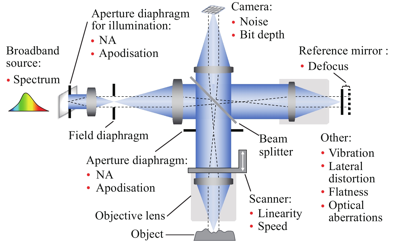
Fig. 2 Schematic setup of a CSI.
Red bullet points indicate influence factors.In this work, we consider a CSI that acquires the 3D interferogram as a stack of 2D images by scanning the object along the optical axis through the focal plane of the imaging objective lens. An axial scan can be carried out using a piezoelectric actuator to move the objective lens with high precision. This scan mode is called “object scanning,” differing from “reference scanning,” in which the reference mirror moves. The fundamental difference between the two scan modes is discussed elsewhere34.
We will use an experimentally determined 3D STF obtained from a real CSI to feed into the virtual instrument and demonstrate the virtual measurement and associated error prediction. Because the 3D STF contains information about the light-source spectrum, NA, pupil apodisation, central obscuration of the Mirau objective, defocus, and other high-order optical aberrations, we need not rely on the nominal values of these instrument parameters when setting up the virtual instrument.
Other major influence factors that are considered in this work include the shot noise and bit depth of the camera, linearity and speed of the actuator, vibration, and lateral distortion and flatness error. The models to incorporate these factors into the virtual measurement will be described in section “Models for incorporating influence factors”. The list of influence factors can be extended within this virtual framework to account for the sources of uncertainty for a specific instrument type and measurement task.
-
A breakdown of the virtual measurement process is provided in Fig. 3. Part I is the 3D interferogram generation, which resembles the 3D stack of interference images that can be obtained from a real instrument. The generation of the complex-valued 3D interferogram
$ O\left({\bf{r}}\right) $ is one of the major advantages of our virtual CSI, because the effects of the influence factors can be directly incorporated into the 3D interferogram. A Monte Carlo method is used to incorporate camera noise and vibration in repeated virtual measurements.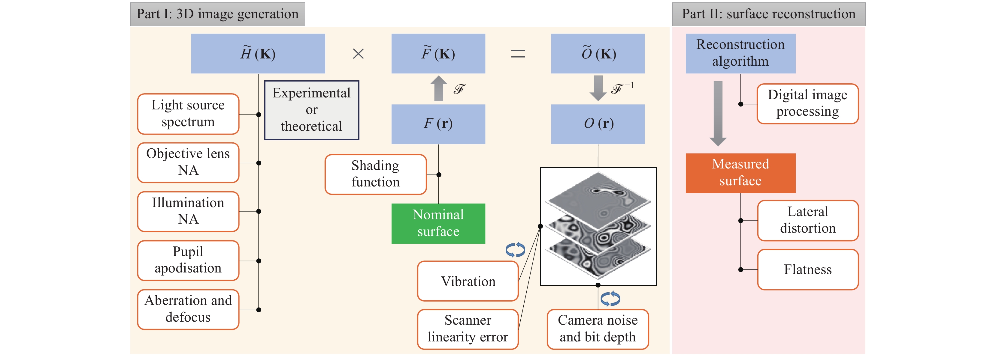
Fig. 3 Breakdown of the virtual CSI measurement process.
In Part II, the final virtual-measurement result is obtained by reconstructing the surface from the 3D interferogram. Any surface-reconstruction method suitable for processing CSI data can be used32. This part of the virtual instrument can be most realistically emulated by using the actual instrument data-processing software, provided that it accepts synthetically generated interference signals from the imaging model.
In this work, we use the frequency-domain analysis (FDA) method41. The FDA method uses both the coherence envelope and the phase of the fringe to calculate the surface height. If a surface-reconstruction algorithm calculates the surface height pixel-wise – i.e. the surface height at each lateral coordinate is calculated by processing the 1D fringe data recorded by the corresponding camera pixel-then, the lateral distortion and flatness error (usually within a few nanometres in a state-of-the-art CSI instrument) can be efficiently applied to the final surface-height map, instead of the 3D interferogram. The simulated 3D interferogram can also be used as a software measurement standard to evaluate the performance of different reconstruction algorithms.
-
If the reference mirror is shifted (in the axial direction) by a distance
$ \varDelta z $ away from the conjugate focal plane of the objective lens (see Fig. 2), the CSI is defocused27,34. In this case, the 3D pupil function for the reference path is written as$$ {\tilde G }_{NA}^{\left({\rm{def}}\right)}\left({\bf{k}}\right)={\tilde G }_{NA}\left({\bf{k}}\right){e}^{i2\varDelta z{\bf{k}}\cdot \widehat{\bf{z}}} $$ (9) and the 3D STF is written as
$$ \tilde H \left({\bf{K}}\right)=\frac{{{\bf{K}}}^{2}}{16{{\text{π}} }^{3}{K}_{z}}\int \int {\tilde G }_{NA}\left({\bf{K}}-{\bf{K}}',{k}_{0}\right){\tilde G }_{NA}^{\left({\rm{def}}\right)}\left({\bf{K}}',{k}_{0}\right){d}^{3}{K}^{'}\frac{S\left({k}_{0}\right)}{{k}_{0}}d{k}_{0} $$ (10) Detailed analyses of defocus in CSIs can be found elsewhere27,34.
-
The linearity error (i.e. positioning error) of the piezoelectric actuator leads to an error in the optical path length between the surface and the objective lens. This error effectively causes a phase shift in the 2D interferogram, which should ideally be recorded at the nominal scan position. At the time when the 2D interferogram is recorded, the phase shift is a constant across the FOV and can be expressed as
$$ {\phi }_{l}\left[{z}_{l}\left({r}_{z}\right)\right]=\;2\frac{{k}_{0}}{q}{z}_{l}\left({r}_{z}\right) $$ (11) where
$ q $ is the NA factor (also known as the obliquity factor) and leads to the equivalent wavenumber$ {k}_{0}/q $ 36. The linearity error$ {z}_{l} $ is calculated as follows:$$ {z}_{l}\left({r}_{z}\right)={z}_{out}\left({r}_{z}\right)-{z}_{in}\left({r}_{z}\right) $$ (12) where
$ {r}_{z} $ is the global coordinate along the optical axis,$ {z}_{in} $ is the nominal input-scan position, and$ {z}_{out} $ is the actual output-scan position. If the actuator drives the objective lens upwards (see Fig. 2) during the measurement, the first 2D image is acquired at scan position$ {z}_{out}={z}_{in}=0 $ , and ideally, the subsequent images should be acquired at$ {z}_{out}\left({r}_{z}\right)={z}_{in}\left({r}_{z}\right) $ . In the presence of linearity error, the subsequent images were acquired at$ {z}_{out}\left({r}_{z}\right)={z}_{in}\left({r}_{z}\right)+ $ $ {z}_{l}\left({r}_{z}\right) $ . Thus, the complex-valued 3D interferogram is multiplied by an additional phase term,$$ {O}^{'}\left({\bf{r}}\right)=O\left({\bf{r}}\right){e}^{i{\phi }_{l}\left[{z}_{l}\left({r}_{z}\right)\right]} $$ (13) -
Vibration may cause the rapidly changing displacement of an object relative to the instrument, and consequently generate measurement errors and noise42. Similar to the effect of the actuator linearity error, this relative displacement causes phase shifts of the 2D interferograms during a measurement. Given the spectrum of the vibration and the scanning speed, the displacement as a function of the scan position can be obtained.
The amplitude-spectrum density of the vibration can be measured in different manners, e.g. by a laser vibrometer. Assuming that the phase of each frequency component in the vibration spectrum is random, the complex-valued amplitude-spectrum density of a vibration can be obtained as
$$ {S}_{v}\left(f\right)={A}_{v}\left(f\right){e}^{i\varphi \left(f\right)} $$ (14) where the measured amplitude-spectrum density
$ {A}_{v}\left(f\right) $ is real-valued,$ f $ is the temporal frequency, and$ \varphi \left(f\right) $ is the random phase (uniformly sampled between 0 and$ 2{\text{π}} $ ) for each frequency.Taking the real part of the inverse Fourier transform of
$ {S}_{v}\left(f\right) $ produces a randomly generated vibration as a function of time. As the axial coordinate$ {r}_{z}={v}_{s}t $ , where$ {v}_{s} $ is the scanning speed, the axial displacement owing to vibration can be written as$$ {z}_{v}\left({r}_{z}\right)={\rm{Re}}\left\{{\int }_{-{\infty }}^{{\infty }}{S}_{v}\left(f\right){e}^{i2{\text{π}} f{r}_{z}/{v}_{s}}df\right\} $$ (15) Then, the complex-valued 3D interferogram can be modified by multiplying by an additional phase term,
$$ {O}^{'}\left({\bf{r}}\right)=O\left({\bf{r}}\right){e}^{i{\phi }_{v}\left[{z}_{v}\left({r}_{z}\right)\right]} $$ (16) where
$$ {\phi }_{v}\left[{z}_{v}\left({r}_{z}\right)\right]=\;2\frac{{k}_{0}}{q}{z}_{v}\left({r}_{z}\right) $$ (17) For every virtual measurement, a new random phase
$ \varphi \left(f\right) $ is generated, such that the phase-shift term$ {\phi }_{v}\left[{z}_{v}\left({r}_{z}\right)\right] $ is different, effectively resulting in a Monte Carlo approach. -
The 3D interferogram term,
$ O\left({\bf{r}}\right) $ , in Eq. 2 is complex. After the effects of some influence factors are incorporated into$ O\left({\bf{r}}\right) $ , its real part is taken to generate the 3D interferogram$ I\left({\bf{r}}\right) $ . According to the bit depth of commonly used cameras in CSI, the floating-point numbers of the measured$ I\left({\bf{r}}\right) $ are rounded to 8-bit or 16-bit integer numbers. By assuming the dominance of shot noise over other noise sources in the camera, the camera noise will be correlated with the intensity value of the interferogram. We estimate camera noise as$$ N\left({\bf{r}}\right)=\alpha {R}_{N}\left({\bf{r}}\right)I\left({\bf{r}}\right) $$ (18) where
$ \alpha $ is a weighting factor that takes a value in the range [0, 1] and$ {R}_{N}\left({\bf{r}}\right) $ is a uniformly distributed random number within [−1, 1]. In a CSI, the noise value is usually smaller than 10% of the signal43, corresponding to$ \alpha <0.1 $ . Based on Eq. 18, the noise is zero if a camera pixel does not receive light (the dark current is assumed to be negligible). The 3D interferogram in the presence of noise is$$ I'\left({\bf{r}}\right)=I\left({\bf{r}}\right)+N\left({\bf{r}}\right) $$ (19) -
Lateral optical distortion causes field-dependent systematic errors in surface measurements. Lateral distortion in a CSI can be calibrated and adjusted by using an areal cross-grating artefact44 or through a self-calibration technique45. The measured distortion can be expressed by a polynomial function; e.g. of the third order. Then, the inverse of the distortion function gives the distortion-correction function. The correction can be carried out on the interferogram or the final topography data, and the corrected interferogram or topography is resampled using interpolation so that it has equi-spaced lateral coordinates.
Residual flatness is systematic and mainly caused by optical aberrations, e.g. field curvature, in the instrument46. The residual-flatness measurements were performed on a calibrated flat reference surface47,48. The residual flatness of a well-calibrated CSI is usually within a few nanometres over an FOV of the order of a millimetre47. In the following analysis, the residual flatness was considered negligible.
-
To demonstrate the effects of the major influence factors on a CSI surface measurement, we set up a virtual CSI with the configuration in Table 1. Unless otherwise stated, this configuration is used throughout this section.
Central wavelength Width of Gaussian spectrum* NA** Pupil apodisation Camera bit depth Scan speed 570 nm 80 nm 0.55 Perfect aplanatic 16 bits 13.4 µm/s * Full width at half maximum (FWHM)
** NA for objective lens; fully filled illumination pupil is assumed. An NA value of 0.15 is also used in some cases.Table 1. Configuration of the virtual CSI
For a fully filled illumination pupil, the NA of the objective lens restricts the maximum angle of both illumination and observation (see Eq. 6). We demonstrate the effects of the NA on the 3D STF, PSF, interferogram, and virtual surface-measurement results in Fig. 4. Two NA values, 0.55 and 0.15, were used for comparison. A sinusoidal surface with a period of 10 µm and a PV of 0.3 µm was virtually measured. The instrument is assumed to be diffraction-limited and free of camera noise, actuator linearity error, and vibration. As shown in Fig. 4, a larger NA offers a larger spatial bandwidth, a narrower PSF, a higher fringe contrast in sloped surface regions, and, consequently, a smaller tilt- and curvature-dependent measurement error.
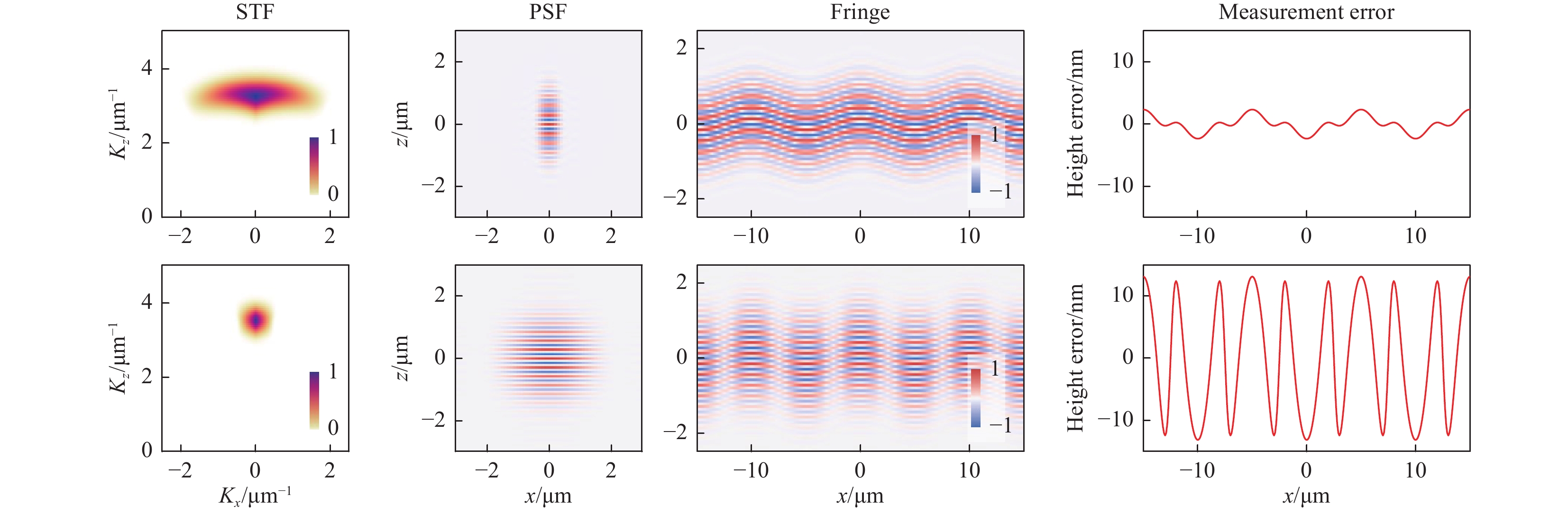
Fig. 4 Effect of NA on the 3D STF, PSF, interferogram, and virtual surface-measurement result.
The central cross-sectional slices in the x-z plane of the 3D data are displayed. Top row: NA 0.55; bottom row: NA 0.15.To demonstrate the effects of defocus, we used a virtual instrument to measure the sinusoidal surface used in Fig. 4. The virtual measurements were carried out in the absence of camera noise, actuator linearity error, and vibration. Two defocus conditions,
$ \varDelta z\;= $ 1 µm and 2 µm, were compared. As shown in Fig. 5, defocus in the CSI reduces the instrument bandwidth, broadens the PSF, and introduces a translational shift to the fringe along the axial direction. Consequently, the measurement error (for non-flat surfaces) is increased.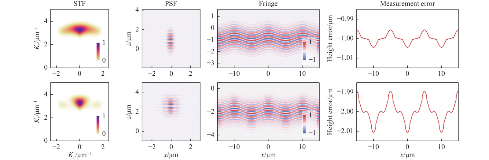
Fig. 5 Effect of defocus on the 3D STF, PSF, interferogram, and virtual surface-measurement result.
Top row:$ \varDelta z=1 $ $ \varDelta z=2 $ The effect of camera noise is demonstrated for the cases of
$ \alpha =0, 0.05,\;{\rm{and}}\;0.1 $ ($ \alpha $ is defined in Eq. 18). The fringe and measurement error for a flat surface are shown in Fig. 6. The instrument is assumed to be diffraction-limited and free of actuator linearity error and vibration. The topographic measurement noise was 0.2 nm for$ \alpha =0.05 $ and 0.4 nm for$ \alpha =0.1 $ . This result is on the same order of magnitude as that found with real instruments42.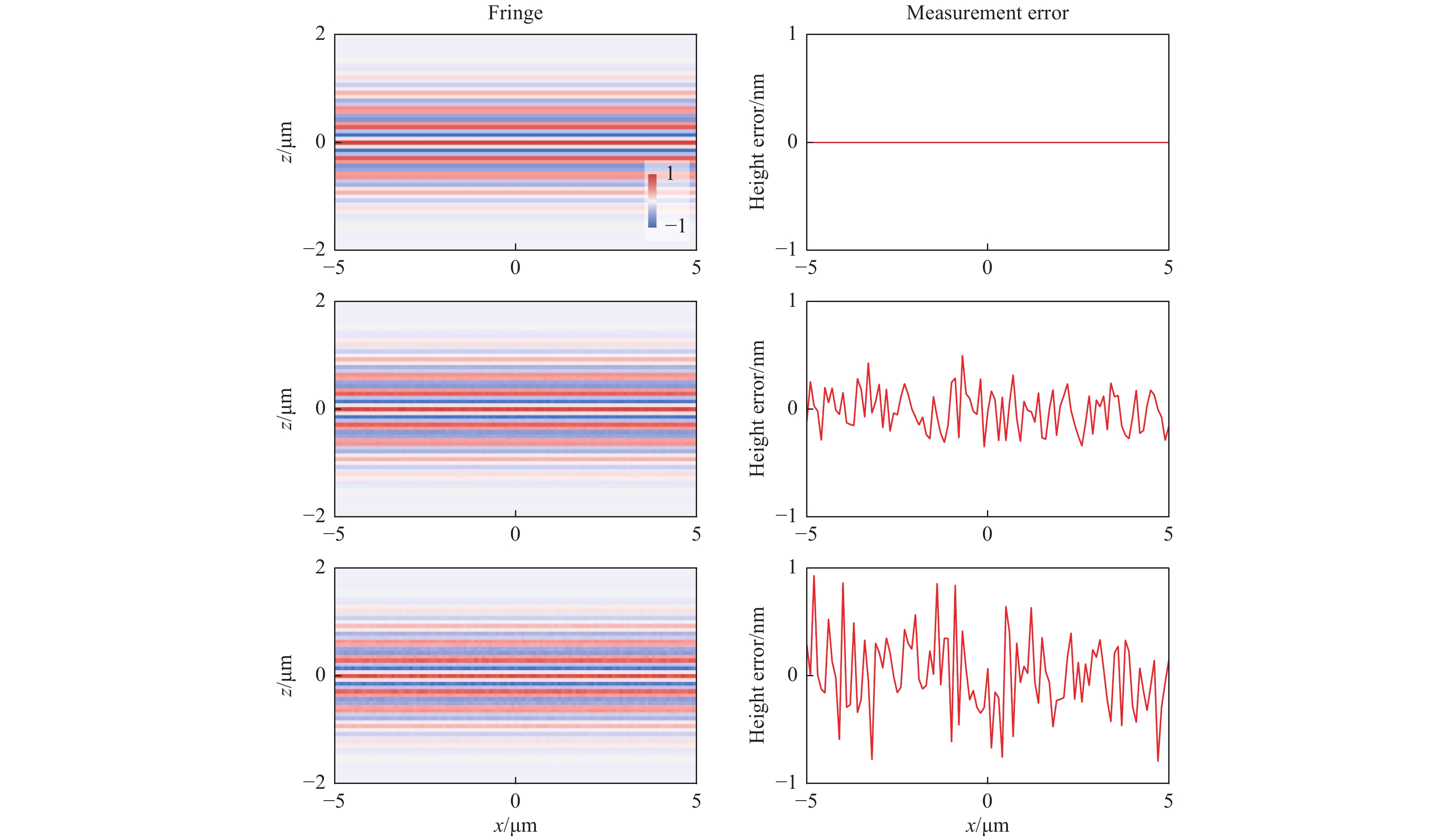
Fig. 6 Effect of shot noise on interferogram and virtual surface-measurement result.
Top row:$ \alpha =0 $ $ \alpha =0.05 $ $ \alpha =0.1 $ The effect of actuator linearity is demonstrated by measuring a flat surface tilted at 10°. The instrument is assumed to be diffraction-limited and free of camera noise and vibration. An arbitrary linearity error is simulated, as shown in Fig. 7a. The measurement error correlates with the linearity error (Fig. 7c). As the positive z direction is defined pointing upwards (see Fig. 2) and the actuator moves upwards in a measurement, a positive linearity error means a longer distance between the objective lens and the surface, which results in a negative measurement error; i.e. the virtually measured surface is below the nominal surface.
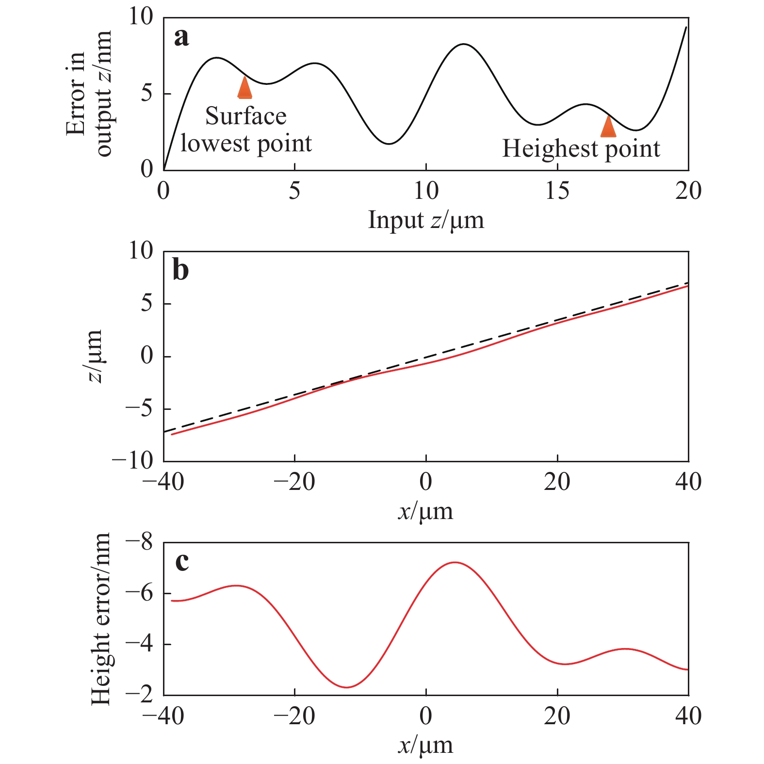
Fig. 7 Effect of actuator linearity on surface measurement.
a Simulated linearity error of the actuator. b Profile of the virtually measured flat surface tilted at 10°. The dashed black line is the nominal surface and the solid red line shows the virtually measured surface, with the error magnified by a factor of 100. c Measurement error.The vibration effect is demonstrated by measuring a flat surface tilted at 4°. The instrument is assumed to be diffraction-limited and free of camera noise and actuator linearity error. The vibration-amplitude spectrum (Fig. 8a) was experimentally measured in a metrology laboratory at the University of Nottingham (this information is used in the virtual measurements in section “Proof of concept”). The spectrum shows a resonance peak at 84 Hz, which is probably produced by a cooling fan in the laboratory42. The randomly generated vibration profile, as a function of the axial coordinate, is calculated based on Eq. 15 (see Fig. 8b). The root-mean-square surface-height error of the virtual measurement is 0.2 nm and is on the same order of magnitude as the topographic noise observed in real measurements42. The noise in real measurements is slightly higher, mainly owing to the presence of camera noise.
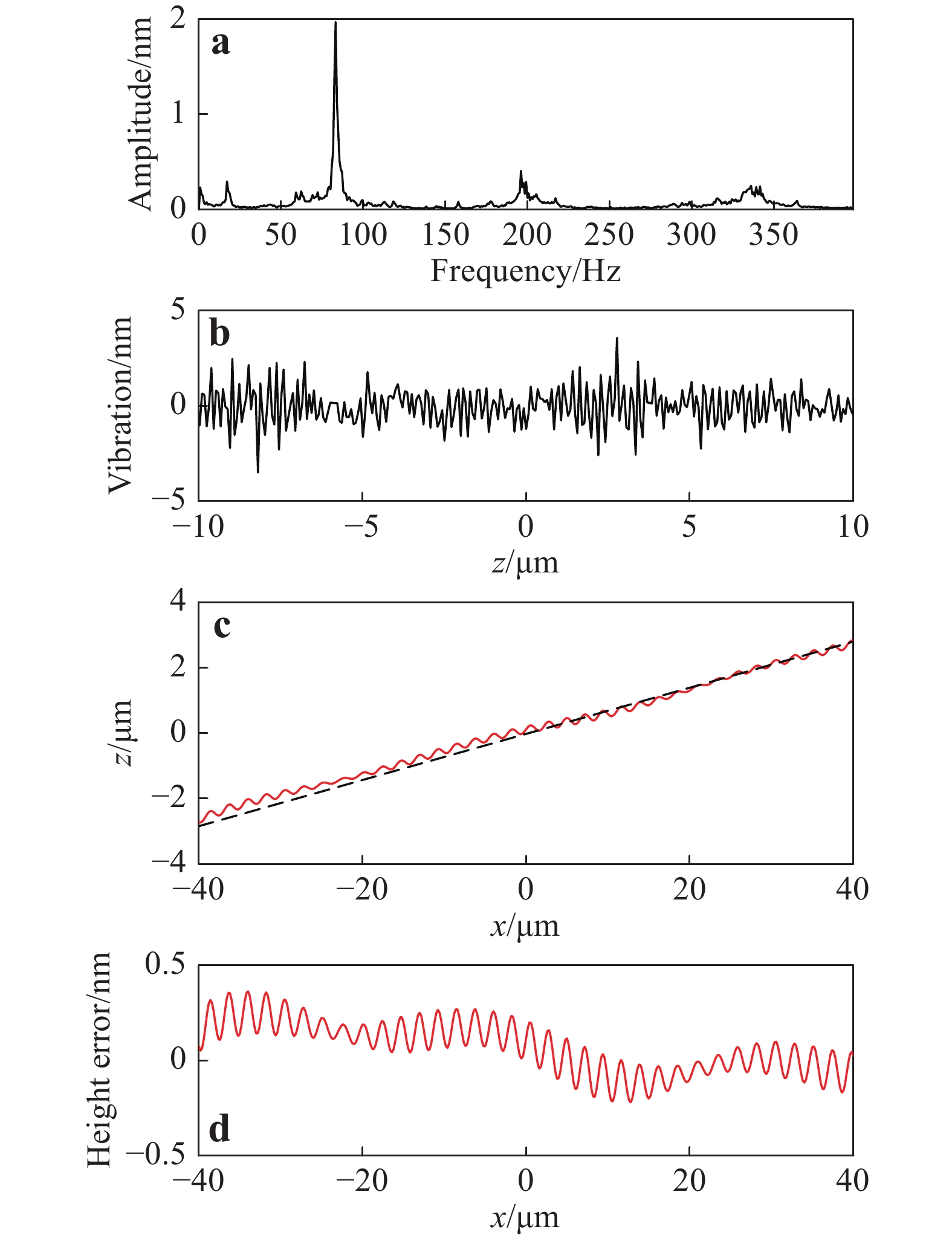
Fig. 8 Effect of vibration on surface measurement.
a Vibration-amplitude spectrum. b Randomly generated vibration. c Central profile of the virtually measured flat surface tilted at 4°. The dashed black line is the nominal surface and the solid red line shows the virtually measured surface, with the error magnified by a factor of 1000. d Measurement error.Unlike the effect of actuator linearity error, the vibration-induced measurement error (Fig. 8d) does not directly correlate with the vibration profile (Fig. 8b). This is because the vibration causes a rapidly changing phase in the interferogram, and the effect of this phase oscillation on surface-height determination is averaged out, when tens of sample points are taken from a fringe to calculate the surface height.
-
We first validate the virtual CSI by comparing its virtual measurement result with that obtained from a real CSI measurement. Then, we will demonstrate the virtual measurements and error predictions for several typical surfaces.
-
The major parameters of the real CSI instrument (equipped with a Mirau objective) are shown in Table 2. The piezoelectric actuator of the instrument was calibrated and adjusted; thus, the residual linearity error was considered negligible. The lateral distortion and flatness were measured and adjusted. The instrument noise is on the order of 0.1 nm.
Central wavelength ~ 570 nm Spectral width (FWHM) ~ 80 nm NA (Mirau objective) 0.55 Lateral sampling distance 174 nm FOV 174 μm Camera bit depth 8 bits Scan speed 13.4 μm/s Table 2. Configuration of the real CSI
The 3D STF of the real CSI is characterised using a method (using a microsphere artefact) discussed38 and validated elsewhere39,49. Considering that a real CSI is never completely shift-invariant, the 3D STF is characterised locally for three regions (west, central, and east; see Fig. 9) within the FOV39. Depending on the degree of shift variance, the FOV can be divided into any number of local regions. We found that three local regions were sufficient for measuring prismatic surfaces using our instrument39.
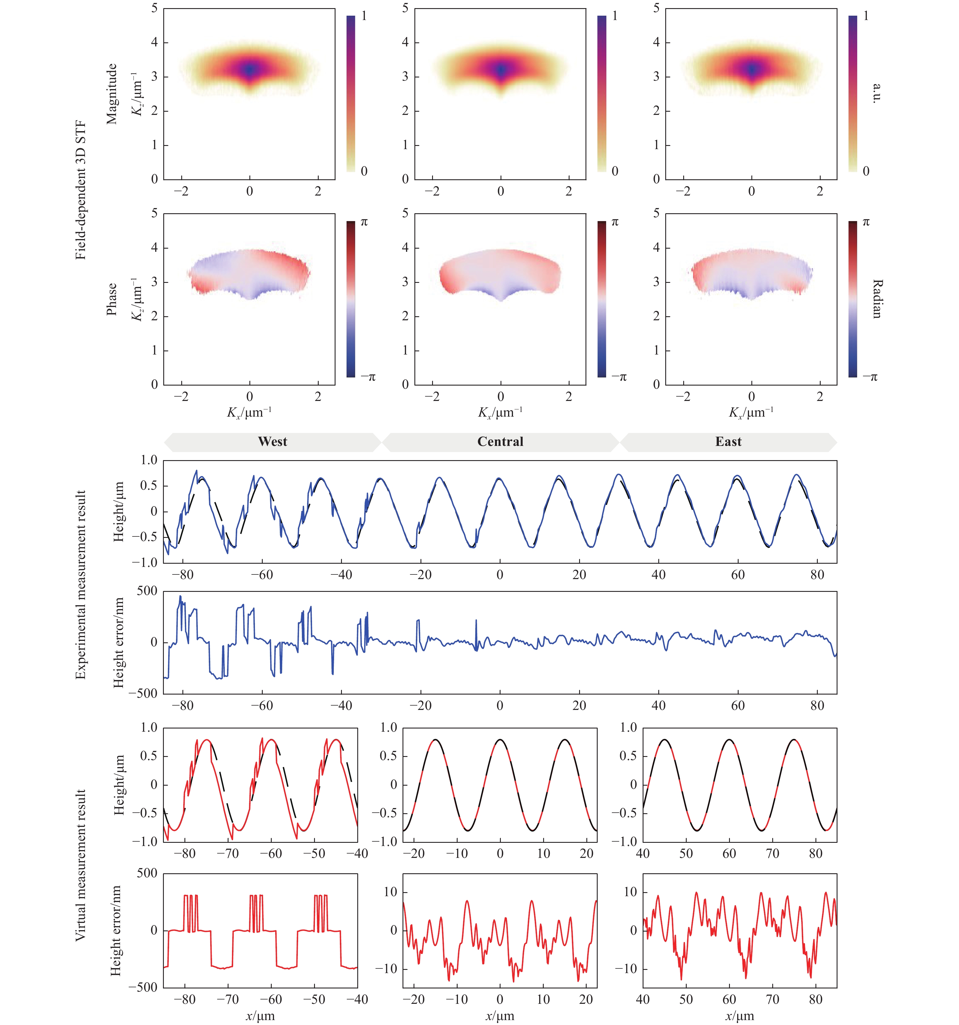
Fig. 9 Comparison between the real and virtual measurements.
The central cross-sectional slices of the field-dependent 3D STFs are shown at the top. The real and virtual CSI results are shown in blue and red lines, respectively.The virtual CSI is set up, based on the field-dependent 3D STFs, the configuration of the real instrument (source spectrum and NA are not needed), and the experimentally determined camera noise and vibration (see section, “Effects of major influence factors”). The actuator linearity error, lateral distortion, and flatness error are considered negligible.
The surface is sinusoidal with a nominal period of 15 µm and a peak-to-valley (PV) of 1.6 µm (a material measure manufactured by Rubert & Co., Ltd.). A reference measurement was made using a calibrated stylus instrument (Talysurf Intra 50) with a 2 µm stylus-tip radius39. As the surface is prismatic and repeatable along the x-direction, the CSI and stylus measurements were made in the same region, but not exactly the same location. The CSI and stylus measurement results were aligned and compared (Fig. 9).
The errors in the CSI measurement are field-dependent, as the instrument is not completely shift-invariant. In general, slope- and curvature-dependent errors are present over the FOV. On the west side, the phase of the 3D STF is significantly distorted, meaning that different spectral components of the foil model of the surface may experience different phases during the imaging process. In real space, the phase distortion deforms the 3D PSF. Consequently, an incorrect estimation of the fringe order by approximately half the mean wavelength may occur, giving rise to the so-called
$ 2{\text{π}} $ errors50.On the east side, the discrepancies in the results near the peaks of the sine wave are likely due to the fact that the measurements are not made at exactly the same location. A more extensive discussion of this comparison process and an evaluation of the resulting measurement uncertainties can be found elsewhere39.
The virtual measurement result is deterministic and can be directly compared to the nominal surface without any alignment to provide position-dependent error maps. As shown in Fig. 9, on the west side of the FOV,
$ 2{\text{π}} $ errors (on the order of 300 nm) on the slopes are accurately predicted in terms of both magnitude and location. The virtual results on the central and eastern sides also agree well with the experimental results. No major$ 2{\text{π}} $ errors occur in these two regions, while the slope- and curvature-dependent errors are slightly higher in the east.Discrepancies between the virtual and real measurements are mainly owing to the following.
1) The real surface topography deviates from the nominal topography and may vary from region to region.
2) The real CSI measurement can only be compared with the reference-stylus measurement because the exact topography of the real surface is generally unknown. Although the stylus instrument has been calibrated and the tip radius of the stylus is much smaller than the pitch of the surface structure, measurement uncertainty still exists9. The repeatability of the stylus measurement was 30 nm (one standard-deviation value) over a 500 µm profile39. However, in the virtual measurement, the result is directly compared to the reference.
3) The 3D STF is field-dependent and varies continuously. We can only assume the shift-invariant condition within a region of the FOV.
4) Surface-reconstruction algorithms may have small variations in their realisation, although both are based on the FDA method.
We can conclude that the virtual measurement mimics the physical measurement with high fidelity, so long as the surface geometry is within the validity regime of the model.
-
Several surfaces were virtually measured using the virtual CSI, including 1) a flat surface levelled and tilted by 4°; 2) a spherical surface with a radius of 30 µm; 3) a sinusoidal surface with a period of 10 µm and a PV amplitude of 1 µm; and 4) a rough surface with an Sq (the areal texture parameter that represents the root-mean-square surface-height values within the definition area) of 150 nm. (The amplitude spectrum of the rough surface has a Gaussian distribution with a standard deviation of 1/3 µm−1. The amplitude spectrum can be calculated from the Fourier transform of the surface topography.)
The virtual instrument was set up in the manner described in the preceding section. The experimentally measured 3D STF of the central region of the FOV (see Fig. 9) was used. Each surface was virtually measured ten times, and the mean topography and standard deviation (
$ \sigma $ ) were calculated. The position-dependent systematic error is obtained by subtracting the nominal surface from the mean surface. The position-dependent repeatability was calculated as$ 2\sigma $ of the ten repeated virtual measurements for each surface point. It should be noted that it is the mean surface, not the nominal surface, which is found within the$ \pm\; 2\sigma $ bounds. In the presence of systematic errors, the mean surface may significantly deviate from the nominal surface.Without any advanced optimisation of computational efficiency, each virtual measurement (40 µm FOV) takes no more than 30 s using a PC configured with an Intel Xeon CPU (E5-1620 v2 @ 3.70 GHz), a 64 GB memory, and a 64-bit operating system.
The direct result of the virtual measurement for the level flat is the surface topography (Fig. 10). Calculation of surface parameters from the surface topography can be considered as a separate process which is relatively easy and optional. Here, we choose Sq as an example. The Sq of the mean topography was 0.04 nm. In this case, the Sq of a level flat corresponds to the measurement noise. This result is consistent with the experimentally evaluated noise reported elsewhere42.
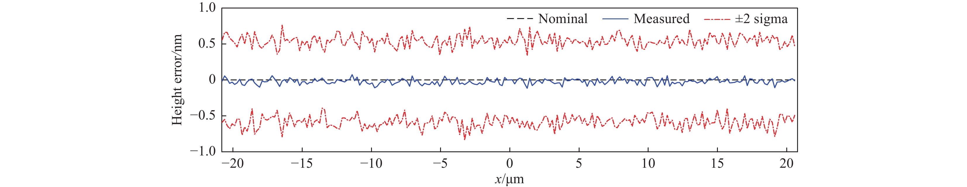
Fig. 10 Mean virtual measurement result and the
$\bf \pm\; 2\sigma $ bounds for the level flat.The profile along the$ x $ $ y{\bf {=0}} $ With a 4° tilt, the vibration effect was observed (Fig. 11). The measurement noise is calculated as the Sq of the error of the mean topography (Fig. 11b), and the result, Sq = 0.12 nm, is again consistent with the experimental result42.
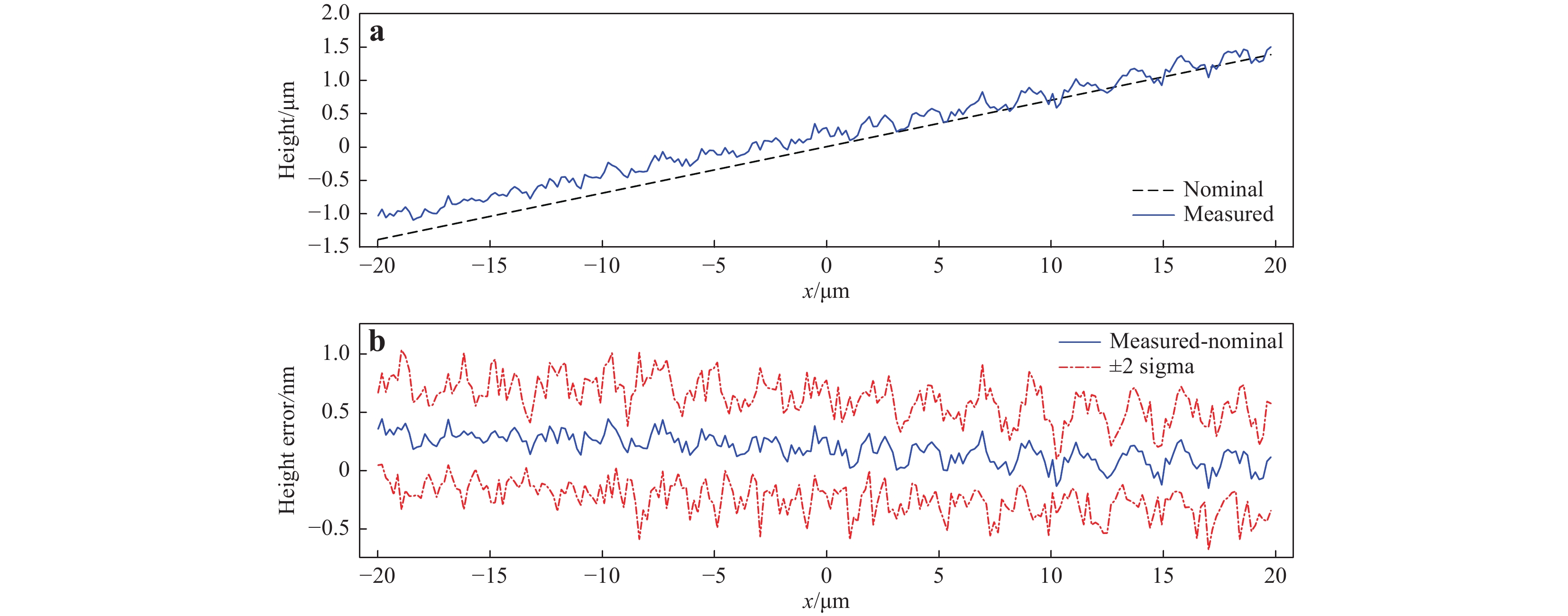
Fig. 11 Virtual measurement result for the flat with a 4° tilt.
a The nominal surface and the mean virtually measured surface (the height error is magnified by a factor of 1000). b The mean virtual measurement error and the$ \pm\, 2\sigma $ $ x $ $ y=0 $ A perfectly smooth spherical surface with a 30 µm radius (Fig. 12a) varies slowly on the optical scale and only reflects light in the specular direction. The spherical surface can be virtually measured, up to the point where the slope angle reaches the maximum acceptance angle of the NA. For a 0.55 NA, the maximum acceptance angle is approximately 33° and corresponds to the lateral position
$ x=16.5 $ µm for this sphere. From Fig. 12c, we can see that the surface can be virtually measured close to the NA limit, but cannot reach the limit because of the non-ideal 3D STF (with a reduced bandwidth and additional phase distortion. See Fig. 9). The presence of optical aberrations causes tilt-dependent errors on the order of 20 nm (Fig. 12b, d) and$ 2{\text{π}} $ errors that occur near the edge of the spherical cap when the surface slope is larger than approximately 23° (Fig. 12c).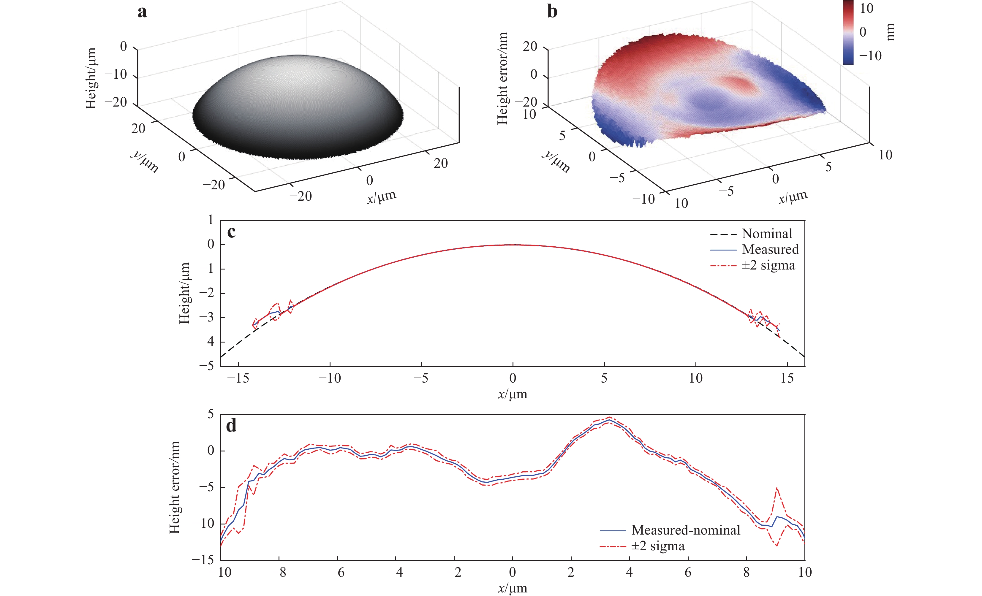
Fig. 12 Virtual measurement result for the spherical surface with a 30 µm radius.
a The nominal surface. b Height error in the mean virtually measured surface. c The central profiles (along the$ x $ $ \pm \,2\sigma $ $ \pm\, 2\sigma $ For the sinusoidal surface (Fig. 13a), we first evaluated whether it satisfied the validity conditions of the Kirchhoff approximation by examining the probability distributions of the surface slopes (Fig. 13b) and the radius of curvature (Fig. 13c). As mentioned in Section, “Basis of the linear theory of CSI”, for dielectric materials, the maximum surface slope should not be so large that the local angles of incidence are larger than 45°. (The Kirchhoff approximation requires that the reflection coefficient
$ R $ is approximately constant for different angles of incidence33,34.) As the maximum surface slope is approximately 17° (Fig. 13b), the slope-angle requirement is satisfied. A sufficiently large radius of local curvature is the most important condition for the validity of the Kirchhoff approximation. We use the criterion defined in Eq. 7 where the coefficient$ {C}_{R} $ must be much larger than unity. As shown in Fig. 13c, this condition is satisfied for this surface.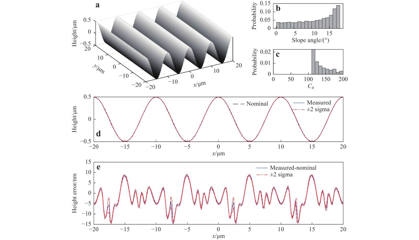
Fig. 13 Virtual measurement result for the sinusoidal surface (10 µm period and 1 µm PV amplitude).
a The nominal surface. b Probability distribution of surface slopes. c Probability distribution of the coefficient$ {C}_{R} $ $ x $ $ \pm\; 2\sigma $ $ \pm\;2\sigma $ The virtual measurement result and position-dependent errors are shown in Fig. 13d, e. Over an FOV of 40 µm × 40 µm,
$ 2{\text{π}} $ errors only occur at 0.15% of the total surface points and only in the regions of negative slopes. The$ 2{\text{π}} $ errors are so sparsely distributed that they are not present in the central profile shown in Fig. 13d, e. In 99.85% of the area, the measurement error (PV value) is within 25 nm. The systematic errors are higher in the valleys (up to 8.8 nm) and negative slopes (−14.4 nm). The value of$ \sigma $ is relatively poor in the high-slope regions, especially the negative slopes, and the maximum value of$ \sigma $ is 2.7 nm (except for areas with$ 2{\text{π}} $ errors). The Sq obtained from the ten repeated virtual measurements is 354 nm ± 0.1 nm, where the uncertainty in Sq is calculated as twice the standard deviation of the ten Sq values. The result is close to the nominal value of 355 nm, and the discrepancy is mainly due to systematic errors.The nominal topography of the Gaussian rough surface is shown in Fig. 14a. In some regions, the local slopes may reach 40° (Fig. 14b). As the maximum slope is still smaller than 45°, the slope-angle requirement is satisfied, even if the material is not a perfect conductor (this point is discussed in Section, “Basis of the linear theory of CSI”). In addition, the coefficient
$ {C}_{R} $ is always larger than 10 for this surface (Fig. 14c).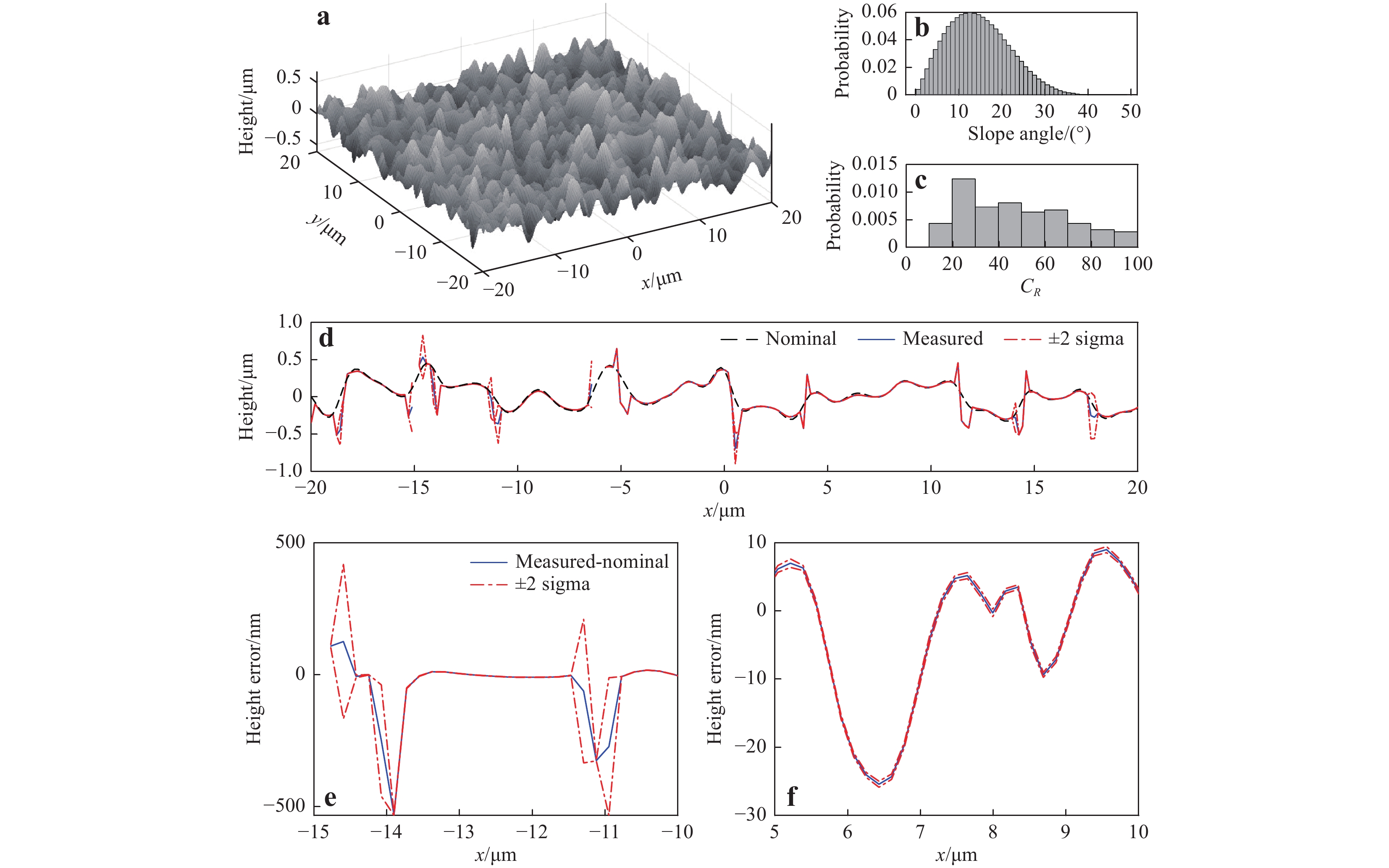
Fig. 14 Virtual measurement result for the Gaussian rough surface (Sq = 150 nm).
a The nominal surface. b Probability distribution of surface slopes. c Probability distribution of the coefficient$ {C}_{R} $ $ x $ $ \pm \;2\sigma $ $ \pm \;2\sigma $ In some high-slope regions,
$ 2{\text{π}} $ errors can be observed. Over an FOV of 40 µm × 40 µm, the mean value of the systematic error is 38 nm and the mean value of$ \sigma $ is 3 nm. The Sq obtained from the ten repeated virtual measurements was 176 nm ± 2 nm. The value is higher than the nominal value (150 nm), mainly due to the presence of$ 2{\text{π}} $ errors and other tilt- and curvature-dependent systematic errors. -
In this paper, we introduced a virtual CSI for surface measurement as a digital twin of a real CSI. The virtual instrument is fully powered by physical models that are derived from first principles. The influences of various error sources were modelled into the 3D interferogram-generation process before the surface was reconstructed. With the a priori information of the 3D surface-transfer function of a real CSI, the virtual measurement mimicked the physical measurement with high fidelity and provided deterministic position-dependent error maps. By repeating the virtual measurement, the statistical information of interest can be obtained. The developed virtual CSI was validated through a comparison with the experimental results of a field-dependent surface measurement.
A virtual CSI can be used to assess the feasibility of an instrument for measuring a specific surface, finding optimal instrument settings, improving the understanding of the measurement process, and testing new instrument configurations. Its primary function is task-specific uncertainty evaluation, which will be discussed in our future work.
The direct result of a virtual measurement is the surface topography, from which the metrological characteristics from ISO 25178 part 600 can be calculated. The metrological characteristics are designed to evaluate uncertainty when it is not possible to gain access to all uncertainty influence factors. The virtual approach is complimentary to metrological characteristics – it is a tool that may also be used to address the term “topography fidelity” (which is mentioned in ISO 25178 part 600, though its assessment is not normative). However, virtual instruments are a different approach, and we will further investigate how the two approaches can be applied together.
By using a surface-scattering model that solves Maxwell’s equations exactly, the virtual CSI can be extended to incorporate multiple-scattering and polarisation effects, which are inevitable with surfaces with complex geometries, e.g. vee-grooves, deep holes, high levels of roughness, and undercuts.
The development of virtual optical instruments will benefit research areas and industries where a quantitative evaluation of surface topography is demanded, e.g. in the areas of tribology, thermal conduction, hydrodynamic control, optics, solar energy, medical implantation, biomimetics, bioelectronics, and microelectronics. This work will also contribute to the advancement of the standardisation of optical surface measurements.
-
The authors would like to thank Prof. Peter de Groot for fruitful technical discussions and reviewing the manuscript. The colour maps used in the figures are released under the CC BY License by Dr Peter Kovesi. This work was supported by the Engineering and Physical Sciences Research Council (EPSRC) [grant numbers EP/M008983/1 and EP/R028826/1].
Physics-based virtual coherence scanning interferometer for surface measurement
-
Rong Su1, 2, ,
 ,
, -
Richard Leach1, ,
- Light: Advanced Manufacturing 2, Article number: 9 (2021)
- Received: 30 October 2020
- Revised: 18 January 2021
- Accepted: 25 February 2021 Published online: 01 April 2021
doi: https://doi.org/10.37188/lam.2021.009
Abstract: Virtual instruments provide task-specific uncertainty evaluation in surface and dimensional metrology. We demonstrate the first virtual coherence scanning interferometer that can accurately predict the results from measurements of surfaces with complex topography using a specific real instrument. The virtual instrument is powered by physical models derived from first principles, including surface-scattering models, three-dimensional imaging theory, and error-generation models. By incorporating the influences of various error sources directly into the interferogram before reconstructing the surface, the virtual instrument works in the same manner as a real instrument. To enhance the fidelity of the virtual measurement, the experimentally determined three-dimensional transfer function of a specific instrument configuration is used to characterise the virtual instrument. Finally, we demonstrate the experimental validation of the virtual instrument, followed by virtual measurements and error predictions for several typical surfaces that are within the validity regime of the physical models.
Research Summary
Virtual optical instruments for traceable surface measurement
The evaluation of uncertainty for optical measurement of surfaces with complex topography (such as freeform and biomimetic surfaces) is an open issue in industrial metrology. A promising approach to uncertainty evaluation is to use a “virtual instrument” – the digital twin of a specific real instrument. Rong Su and Richard Leach from China’s Shanghai Institute of Optics and Fine Mechanics and UK’s University of Nottingham respectively report the first virtual coherence scanning interferometer for surface measurement. The virtual instrument is fully powered by physical models derived from first principles and provides deterministic measurement results for surfaces with complex topography, akin to the results obtained with a real instrument. The software to implement the virtual instrument is made publicly available under the CC BY License.
Software download link: https://doi.org/10.13140/RG.2.2.14658.09922/2


Rights and permissions
Open Access This article is licensed under a Creative Commons Attribution 4.0 International License, which permits use, sharing, adaptation, distribution and reproduction in any medium or format, as long as you give appropriate credit to the original author(s) and the source, provide a link to the Creative Commons license, and indicate if changes were made. The images or other third party material in this article are included in the article′s Creative Commons license, unless indicated otherwise in a credit line to the material. If material is not included in the article′s Creative Commons license and your intended use is not permitted by statutory regulation or exceeds the permitted use, you will need to obtain permission directly from the copyright holder. To view a copy of this license, visit http://creativecommons.org/licenses/by/4.0/.
Software for virtual coherence scanning interferometer (version 1.0 Beta)
Uncertainty evaluation for optical measurement of surfaces with complex topography (such as freeform and biomimetic artificial surfaces) is a long-standing gap in industrial metrology capability. A promising approach to uncertainty evaluation is to use a “virtual instrument” – the digital twin of a specific real instrument. Rong Su and Richard Leach from China’s Shanghai Institute of Optics and Fine Mechanics and UK’s University of Nottingham respectively now report the first virtual coherence scanning interferometer for surface measurement. The virtual instrument is fully powered by physical models derived from first principles and provides deterministic measurement results for surfaces with complex topography as can be obtained using a real instrument. The software to implement the virtual instrument is made publicly available under the CC BY License. Software here: https://doi.org/10.13140/RG.2.2.14658.09922/2

 DownLoad: