Variable shearing holography with applications to phase imaging and metrology

Single-beam wavefront reconstruction techniques are exciting alternatives to interferometry. These techniques are inherently robust to vibrations and often can be designed in a compact optical setup. Recent research expands those techniques to partial coherent sources, where LEDs are employed in place of lasers. Another interesting field is the area of bio-imaging, where existing microscopes are converted into phase measuring devices using a single-beam phase wavefront reconstruction add-on. A further appealing aspect is that many single-beam systems can be designed to work with no beamsplitter, allowing the sensor to be closer to the sample and enabling simpler optical measurements with higher-numerical aperture. In phase retrieval, there are two representative families of wavefront reconstruction techniques. Firstly, techniques based on deterministic models^1–5, and secondly, techniques that employ an iterative solver that utilizes wave-propagation techniques^6,7 or Fourier relationships^8,9.

With the advent of faster computer systems, new cameras are often developed with a higher pixel count, diminishing many advances of the higher computational power. Optical measurement technologies need to adapt to survive this trend through more innovative algorithms, new measurement concepts, or both.

For instance, in the field of phase retrieval, the convergence may be improved using multi-resolution and relaxation techniques¹⁰. Another possibility is to alter the illumination¹¹ or combine deterministic and iterative algorithms¹².

However, the elephant in the room of all methods mentioned above is the inverse problem resulting from the data produced by the unmodulated optical beam. In other words, often, the data is too similar, and significant efforts need to be made to reduce the similarity (e.g., repeating the measurement at a large defocus distance³).

Recent advances in computational shear interferometry^13,14 allow actively modulating an incident beam as it interferes with itself. Modulation of the beam increases instantly the diversity in the data. In particular, when employed with phase-shifting techniques¹⁵, it is possible to obtain the complex crossterm of two interfering wavefields directly. Despite this sophistication, the system by Falldorf¹³ requires a spatial light modular (SLM), which significantly contributes to the system costs. The wavefront reconstruction technique reported by Falldorf et al.¹³ is based on a gradient descent approach for non-symmetric shearing systems. However, compared to the non-symmetric case, deriving the grading of a that non-holomorphic function for the case of a “symmetric” shearing system is not straightforward. Hence other approaches like the alternating projections by Konijnenberg¹⁶ are preferred reconstruction algorithms.

Recent advances in geometric phase (GP) elements lead to the development of GP gratings and GP lenses that can be employed in lateral and radial shearing interferometry^17–19, with polarization phase-shifting capabilities^20,21. The remaining quest is to recover the correct wavefront from the captured phase-shifted interferograms.

This paper proposes a variable shearing interferometer that consists of a series of GP gratings and polarization optics. This setup enables measuring a series of phase-shifted interferograms for a given shear amount, as shown in Fig. 1. In a subsequent step, we reconstruct the wavefield using a modified version of the alternating projections algorithm, developed by Konijnenberg¹⁶, and a series of interferograms with different amounts of shear. The discussed systems are the first experimentally demonstrated GP grating-based variable shear interferometers for complex wavefield reconstructions. We discuss various possible configurations of these instruments and demonstrate the success of two distinct shear selection strategies (employing one or two grating pairs). We analyze these findings using the “frequency information density” and the “spatial information density” analyses based on transfer function and support function concepts introduced by Servín in Ref. 22. We further show that a GP grating configuration with a fixed shear amount, but an adjustable rotational shear axis (one mechanical rotational axis) is sufficient to obtain robust measurements while maintaining phase-shifting capabilities using a pixelated polarization camera. We also investigate the effect of other error sources (e.g., imperfect shear estimation), which affects the resolution of the reconstructed wavefront. This effect is not commonly known (for coherent systems, the resolution is often a result of numerical aperture, pixel size, or spatial coherence of the source). To mitigate this source of error, we report a shear detection technique using the peaks of the second derivative of the autocorrelation function of the holograms. Measuring the shear amount directly from the hologram is different from relying on a well-calibrated system and increases the system’s accuracy.

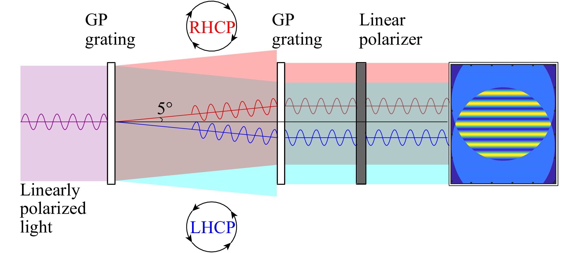
Fig. 1  Principle of GP grating based shearing interferometry for the case of linearly polarized light.

Polarization gratings, also known as geometric phase (GP) gratings, are liquid crystal polymer-based optical gratings with a diffraction angle that depends on the polarization and wavelength of light. GP gratings are designed to diffract right-handed circularly polarized light (RHCP) and left-handed circularly polarized light (LHCP) at a negative angle and positive diffraction angle, respectively. The value of this angle depends on the prescription; commercially available gratings with various groove densities result in diffraction angles of the first-order between 3 and 10 degrees. The diffraction angle can be related directly to the wavelength and groove density using the well-known equation m λ = d sin(θ).

A lateral shear in the spatial domain is achieved when two GP gratings are placed consecutively¹⁷, as shown in Fig. 1. In that configuration, both identical GP gratings are aligned along the same axis and orientation. In this way, the first GP grating deflects the incoming beams at the angles +/− α, and the second GP grating compensates this deflection by diffraction the beam into −/+ α. The properties of these GP gratings in this configuration are outlined in Ref. 17. Adjusting the distance between the first and the second GP grating allows adjusting the shear amount of the two interfering waves, as shown in Fig. 2, enabling unique properties that can be used for adjustable shearing interferometry.

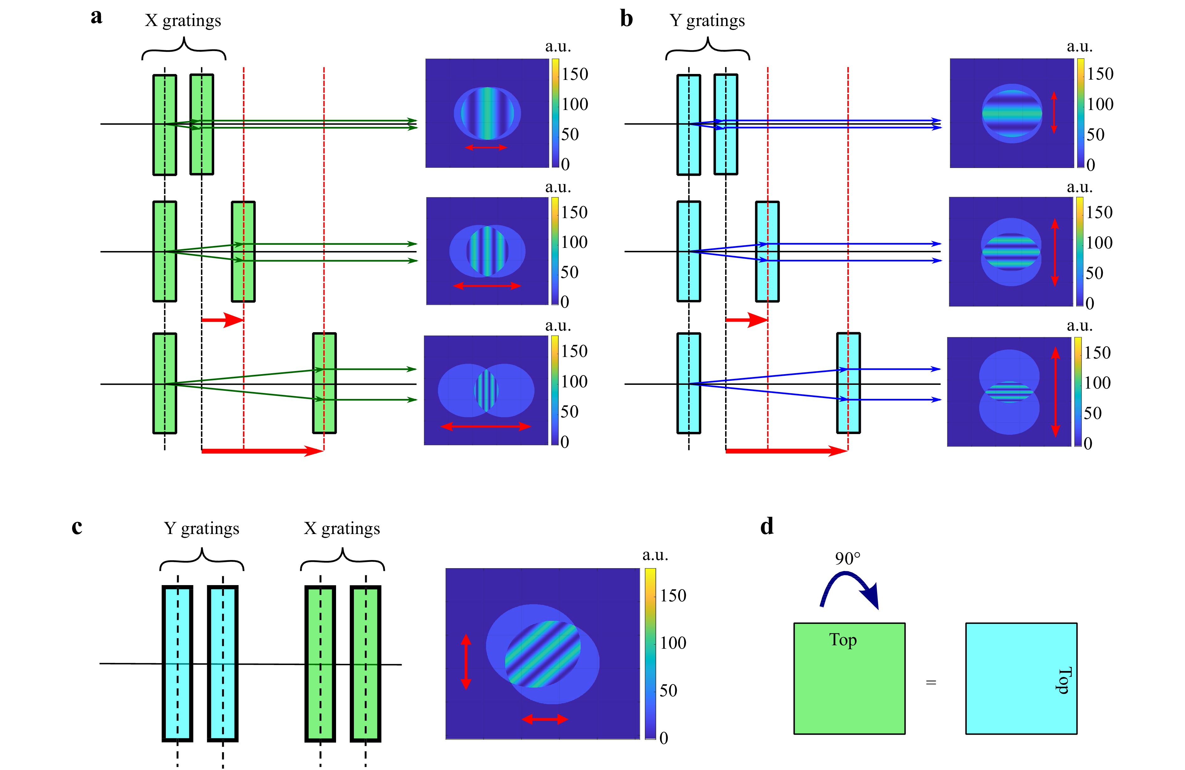
Fig. 2  Examples of interferograms for the case of a spherical wave at the distance z = 350 mm with different shear amounts in x- and y- direction.

As shown in Fig. 2, shearing along the y-axis is possible by flipping the gratings by 90 degrees. An instrument employing a series of four GP gratings enables shearing in both x- and y-direction. This configuration shears along the x- and y-axis independently. This system uses 4 gratings in total: one pair for x-shear and the other pair for y-shear.

A different possible configuration is to maintain a fixed shear between two beams and modulate the fringes by rotating the shear axis about the optical axis, as shown in Fig. 3. This configuration requires only one GP gratings pair and is more compact than the other configuration of Fig. 2c.

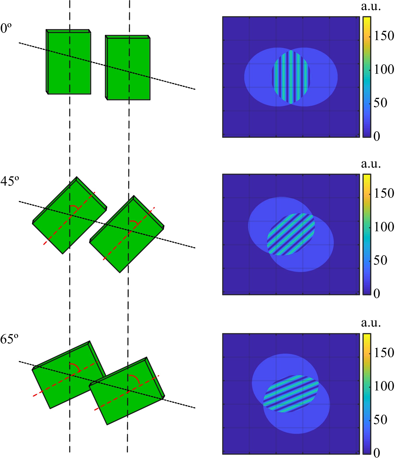
Fig. 3  Examples of interferograms for the case of a spherical wave at the distance z = 250 mm with constant shear and different grating rotational angles.

Furthermore, as the linearly polarized light at the instrument’s input is converted into left and right circular polarized components, there is a need to employ a linear polarizer to make these two waves interfere. Notably, this configuration provides geometric phase-shifting capability²³, i.e., by rotating the axis of the polarizer, it is possible to create a series of phase-shifted interferograms, as shown in Fig. 4.

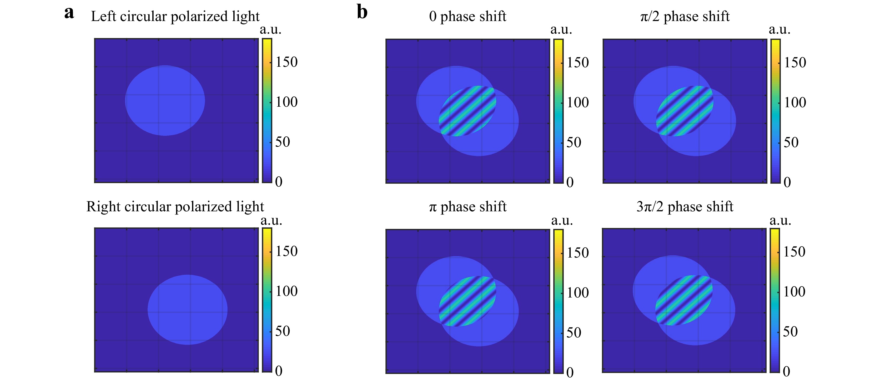
Fig. 4  a Intensity ditribution of a spherical wavefront with constant amplitude before reaching the linear polarizer. b Intensity after the linear polarizer for four different angles of the polarizer axis to produce a phase shift between interfering waves of 0, π/2, π, and 3π/2.

In the following sections, we propose using GP gratings for multi-shear variable shearing interferometry with phase-shifting capability. We further evaluate the performance of the instrument with mentioned above configurations using multi-shear wavefront reconstruction techniques.

The previous section showed how GP gratings could obtain a series of phase-shifted interferograms for various shear amounts. These interferograms allow calculating the complex cross-terms of the two-interfering waves at each shear. The challenge is to reconstruct the complex wavefield from this data. In this section, we present an iterative algorithm based on the approach of Konijnenberg¹⁶ that was inspired by the alternating projection algorithms^9,24.

Consider a general wavefield u with the amplitude A and the phase ϕ as

which produces the following interferogram $ {I}_{n,\delta }\left(\overrightarrow{x}\right) $ in shearing, as

Where $ \overrightarrow{{\rm{d}}{\rm{s}}}=\left[{{\rm{d}}{\rm{s}}}_{{\rm{x}}},{{\rm{d}}{\rm{s}}}_{{\rm{y}}}\right] $ and, $ {{\rm{d}}{\rm{s}}}_{{\rm{x}}} $ and $ {{\rm{d}}{\rm{s}}}_{{\rm{y}}} $ is the shear in x- and y- direction, δ is the phase shift induced by the rotating polarizer, and $ {C}_{n}\left(\overrightarrow{x}\right) $ is the complex cross-term

The term $ {C}_{n}\left(\overrightarrow{x}\right) $ is estimated using phase-shifting techniques, which for the four-bucket algorithm results in

The reconstruction algorithm uses the term $ {C}_{n}\left(\overrightarrow{x}\right) $ that is obtained at different shears ‘$ \overrightarrow{{s}_{n}} $’ to reconstruct the object wavefield through an iterative process. In this work, we employ an alternating projections (AP) approach developed by Konijnenberg¹⁶ for the x-ray community. The algorithm applies two distinct constraint sets, where each constraint allows only a limited family of solutions. The objective of the wavefield reconstruction algorithm is to identify the unique solution that satisfies all constraints (and for all shears). These constraints are satisfied by employing alternating projections between the two solution domains, in which we apply both, so-called “object constraints” and so-called “measurement constraints”.

Switching between “object constraints” and “measurement constraints” is applied continuously until the algorithm converges to a specific wavefield. The convergence can be conveniently estimated using the following loss function

where subscript n denotes that the wavefield uses the shear $ \overrightarrow{d{s}_{n}} $, S is the total number of shears, and for convenience, we define the estimated wavefield after N iterations as $ f\left(\overrightarrow{x}\right) $ to distinguish it from ideal wavefield $ u\left(\overrightarrow{x}\right) $. The notation $ f\left(\overrightarrow{x}\right) $ is used as a general indication to represent estimated wavefields from both constraints, where the notation $ {f}^{M}\left(\overrightarrow{x}\right) $ denotes the estimate of the wavefield directly after the measurement constraint is applied, and $ {f}^{O}\left(\overrightarrow{x}\right) $denotes the estimate of the wavefield directly after the object constraint is applied. For further simplification, the symbols 'n,+' and 'n,-' in the subscript are used to represent positive and negative shears, i.e.,

$ {f}_{n,\pm }\left(\overrightarrow{x}\right)=f\left(\overrightarrow{x}\pm \overrightarrow{d{s}_{n}} \right) $. Consequently, the estimated complex cross amplitude term can be presented as

and can be generated using the estimated wavefield $ {{{\rm{f}}}^{{\rm{M}}}}_{{\rm{n}}}\left(\overrightarrow{{\rm{x}}}\right) $ at any shear $ \overrightarrow{{S}_{n}} $.

Notably, in the presence of noise, there is no exact solution. However, the wavefield reconstruction algorithm estimates the best fit solution that matches the experiment data. The loss function serves as a metric to be observed for convergence with an increasing number of iterations.

Fig. 5 shows the steps of the wavefield reconstruction algorithm. After an initial guess, the algorithm continuously applies the so-called object and measurement constraints alternatingly until the loss function reaches the desired level. The application of those constraints is discussed in more detail below.

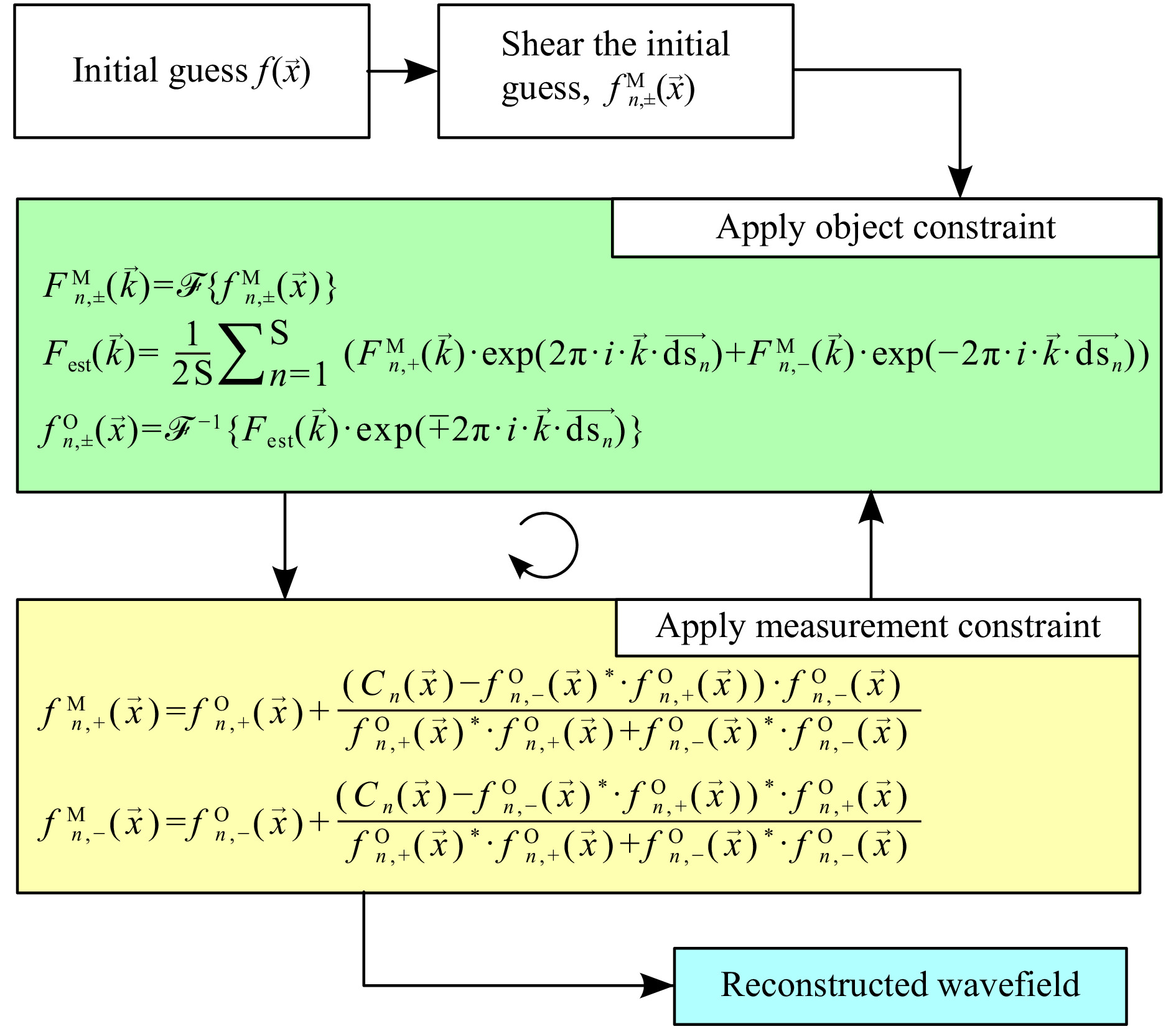
Fig. 5  Principle of multi-shear wavefront reconstruction algorithm.

This step of the algorithm uses only the initial guess $ {\rm{f}}\left(\overrightarrow{{\rm{x}}}\right) $ in the first iteration to estimate $ {{{\rm{f}}}^{{\rm{M}}}_{{\rm{n}},\pm }}\left(\overrightarrow{{\rm{x}}}\right) $. An initial guess is assumed for $ {\rm{f}}\left(\overrightarrow{{\rm{x}}}\right) $ (e.g., a spherical wave, a plane wave, or a random wavefield) and is laterally sheared by the same shears used in the experiment. For a wavefield $ {\rm{f}}\left(\overrightarrow{{\rm{x}}}\right) $, the shearing is done in the Fourier domain using the following equations.

Assuming that the initial guess wavefield is from the measurement constraint domain, the initial guess and its sheared components are indicated as $ {{{\rm{f}}}^{{\rm{M}}}_{{\rm{n}},\pm }}\left(\overrightarrow{{\rm{x}}}\right) $. A wavefield with constant phase and unit amplitude is used as an initial guess for the reconstructions done in this paper.

The object constraints are applied by transforming the sheared components of the estimated wavefield to the Fourier domain and compensating the shear for each $ {{{\rm{f}}}^{{\rm{M}}}_{{\rm{n}},\pm }}\left(\overrightarrow{{\rm{x}}}\right) $ to obtain $ {\rm{f}}\left(\overrightarrow{{\rm{x}}}\right) $ using the Fourier Shift theorem. All calculated values for $ {\rm{F}}\left(\overrightarrow{{\rm{k}}}\right) $ are averaged to obtain a more accurate result.

Finally, $ {{\rm{F}}}_{{\rm{e}}{\rm{s}}{\rm{t}}}\left(\overrightarrow{{\rm{k}}}\right) $ is transformed back into the spatial domain using the inverse Fourier transform. However, because the measurement constraints (applied in the second part of the iteration) require the wavefield for different shears, we apply again the Fourier shift theorem to obtain $ {{{\rm{f}}}^{{\rm{O}}}_{{\rm{n}},\pm }}\left(\overrightarrow{{\rm{x}}}\right) $ as

The measurement constraint equations use the estimated wavefield from the object constraint $ {{{\rm{f}}}^{{\rm{O}}}_{{\rm{n}},\pm }}\left(\overrightarrow{{\rm{x}}}\right) $ and the measured complex cross-term $ {{\rm{C}}}_{{\rm{n}}}\left(\overrightarrow{{\rm{x}}}\right) $(obtained from phase shifting) to estimate the wavefield solution in the measurement constraint domain. The following equations are a modified version of the equations used by Konijnenberg in¹⁶ to estimate the wavefield.

The algorithm uses two sets of constraint equations, object constraint Eq. 10, and measurement constraint Eqs. 12, 13. Each set of constraint equations has a solution set. The algorithm starts with an initial guess projected onto the object constraint solution set by using the respective equations. This produces an estimated wavefield which is a projection on the object constraint solution set. This wavefield is then projected onto the measurement constraint solution set using the respective equations, and the process repeats until convergence. Ideally, the solution we are looking for is the one that is at the intersection of these two solution sets. However, in practice, due to noise and other external factors, such intersection does not exist, and the algorithm converges when the projections oscillate between the two solution sets with solutions at the closest proximity to each other.

The performance of the algorithm was evaluated by simulations using MATLAB. Preliminary simulations were made for a resolution of 256 × 256 pixels. For this simulation, a point source was generated with a wavelength of 600 nm at a z-distance of 87.5 mm and was sampled with a pixel size of 3.45 μm. The reconstruction algorithm uses FFTs to shear the estimated wavefields at different steps in the reconstruction. The use of FFTs, in turn, implicitly imposes a periodic boundary condition. Therefore, we use an aperture for both simulations and experiments to mitigate problems during reconstruction that might arise from periodic properties of FFTs. For this reason, a circular aperture mask with a diameter of 180 pixels was applied. Future reconstruction algorithms may exclude samples that exceed the computational window, especially at larger shear. Those samples need to be reconstructed with measurements taken at smaller shear amounts.

A series of four phase-shifted intensities were generated for each shear position. The shears generated for this simulation are shown in Fig. 6a. Additive white Gaussian noise (AWGN) with a standard deviation of 20% of the peak intensity has been added to the generated intensities to model the effect of noise in these simulations. Afterward, to realistically model the effect of cameras, an 8-bit discretization has been applied to the intensities.

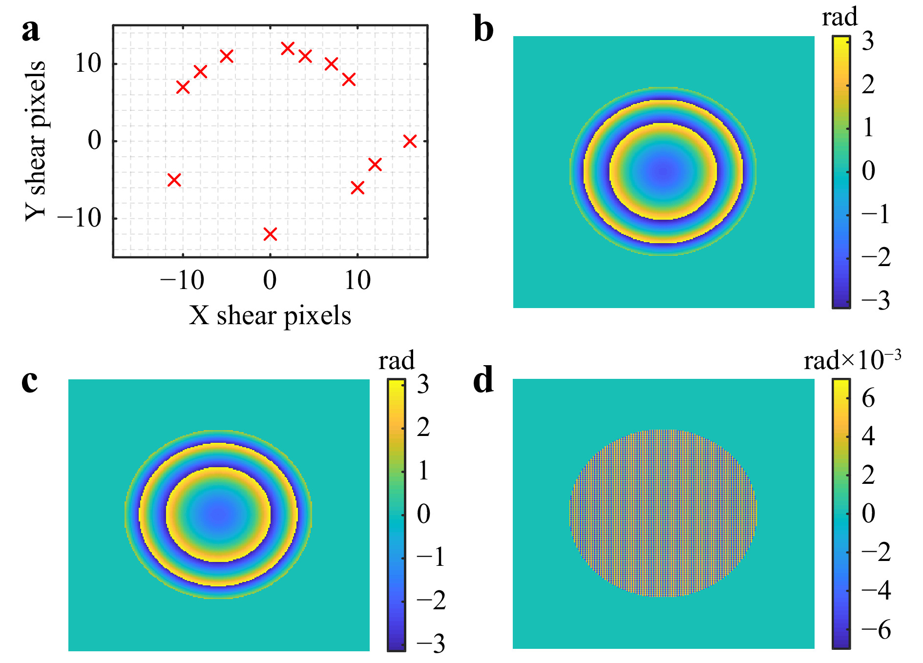
Fig. 6  (Simulation) Results of reconstruction with simulation parameters: FoV 256 × 256 pixels, Pixel size 3.45 μm,Wavelength 0.6 μm, Aperture size 90 pixels, Z distance 87.5 mm. a Shear selection. b Ideal phase map. c Reconstructed phase map. d Error map between ideal and reconstructed data.

For this simulation, a total of 48 interferograms have been generated corresponding to 12 different shears with 4 phase-shifted interferograms. The ideal wavefront and reconstructed wavefront are shown in Fig. 6b, c, respectively. The corresponding phase error of the reconstructed wavefront is shown in Fig. 6d. Further investigation of the error map showed the presence of high-frequency artifacts, as highlighted in Fig. 7.

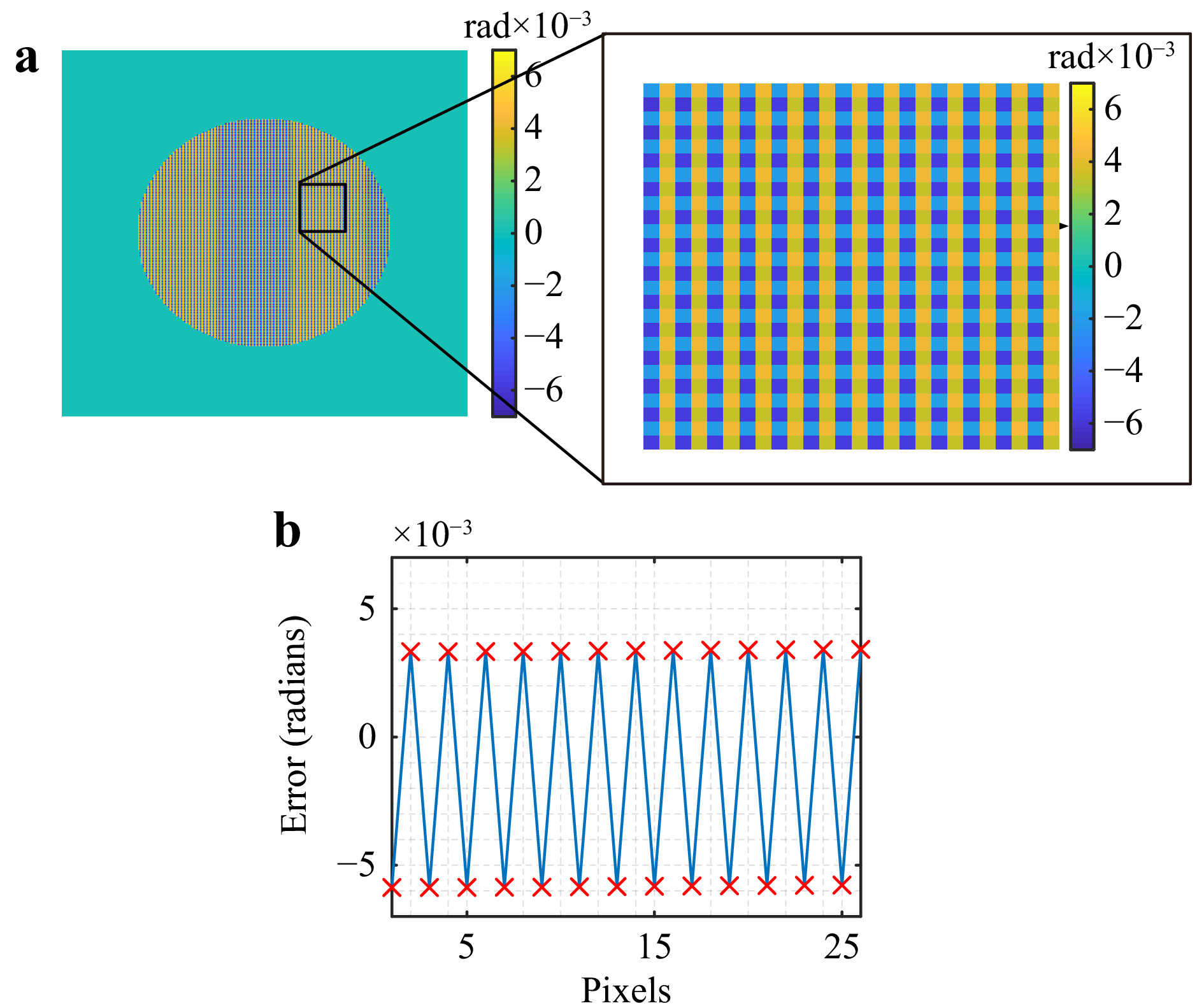
Fig. 7  High frequency artifact from reconstruction algorithm. a Error map zoomed. b Error map profile.

These high-frequency artifacts occur at Nyquist frequency and appear to be a product of the reconstruction algorithm. Further analysis is required to investigate the source of these artifacts. For the reconstructions discussed in this paper, we use a low-pass Fourier filter to mitigate the formation of these artifacts.

Fig. 8 shows error maps generated by mapping the difference between the ideal and reconstructed wavefield before and after applying the filter. A cross-section of the error profile before and after filtering is shown in Fig. 8c, d, respectively. This simple procedure reduces the magnitude of the RMS error by one order of magnitude. Because a Fourier low-pass filter has been employed with a corner frequency of $ {k}_{c}=\left({4}/{5}\right)\cdot \left({1}/{\rm{pixel\;size}}\right) $, an artifact is produced along the boundary of the aperture. However, other filtering techniques may be applicable depending on the application, and even Zernike polynomials may be fitted to the data. The use of different filtering techniques is beyond the scope of this work.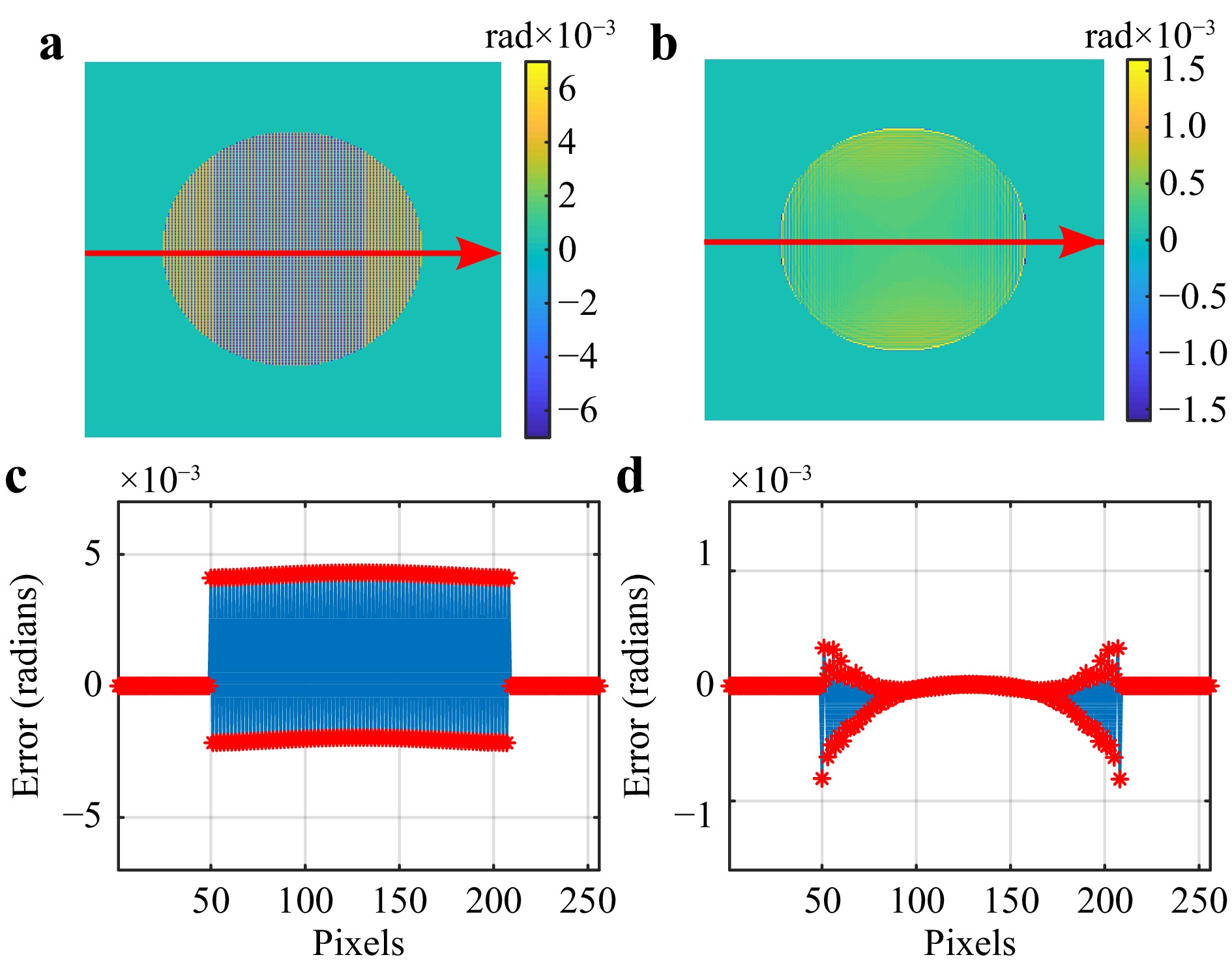

Fig. 8  a Error map before filter (RMS error: 4.1E-3 rad). b Error map after filter (RMS error: 0.42E-3 rad). c Profile of error map before filter. d Profile of error map after filter.

As mentioned earlier, the evolution of the loss function indicates how close the algorithm is to achieving the best solution or achieving convergence. The loss function is evaluated in these experiments by calculating the change between the solutions generated by the two constraints on positive and negative sheared estimated wavefields. The loss function was already defined in Eq. 5 and is reiterated here in Eq. 14 for convenience. Fig. 9a shows the evolution of loss function during reconstructions done in Fig. 8 before the filter was applied.

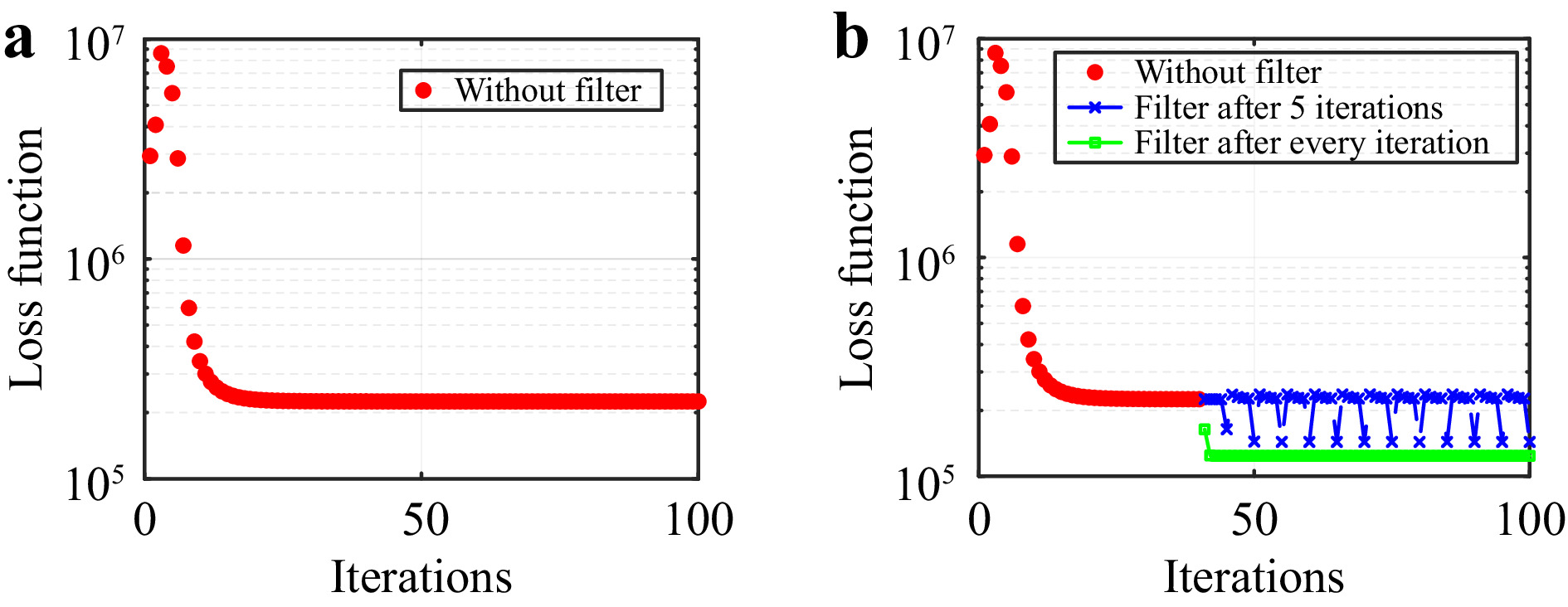
Fig. 9  Evolution of loss function. a without filter. b with filter.

Fig. 9a shows that the loss function converges after 30 iterations of the reconstruction without a Fourier filter. Given the filter’s effectiveness in Fig. 8, we have investigated the use of the filter within the reconstruction algorithm. The sudden surge at the start of the loss function in Fig. 9 is a characteristic feature of phase retrieval and reconstruction algorithms. The temporary increase of the value of the Loss function is expected because the solver climbs out of the local minimum. Other phase retrieval algorithms such as the “hybrid input-output algorithm”⁸ show a similar behavior.

Two cases were considered for this study: (i) using the filter after every 5 iterations and (ii) applying the filter in every iteration. Fig. 9b shows that applying a filter enables a drop in the convergence values in both cases, thus indicating an improvement in the reconstruction process. Interestingly, the reconstruction algorithm for case (i) consistently converges back to the solution containing the high-frequency artifact. Therefore, we recommend employing a Fourier filter within the wavefront reconstruction algorithm to suppress all undesired artifacts continuously.

Please note, the algorithm described is a modified version of the alternating projections algorithm developed by Konijnenberg et al. in Ref. 16. For better clarity we summarize the differences to the original algorithm from Ref. 16.

● The data recorded from experiments in Ref. 16 are in the Fourier domain. In this paper, all recorded data from experiments are in the spatial domain.

● Eq. 10 is the modified version of the object constraint equation. The original equation (Eq. 10 in Ref. 16) was defined in the spatial domain. In this paper, this equation is defined in the Fourier domain.

● Eqs. 12,13 are the modified versions of the measurement constraint equations. The original equations (Eq. 15 in Ref. 16) were defined in the Fourier domain. In this paper, these equations are defined in the spatial domain.

● The algorithm in Ref. 16 uses two sets of equations in measurement constraint (Eqs. 15,16 in Ref. 16), rough-reconstruction equations for initial convergence (Eq. 16 in Ref. 16) and fine-reconstruction equations for final refinement (Eq. 15 in Ref. 16). This paper only uses the modified versions of the fine reconstruction equations.

● After initial convergence, we include a Fourier filter in the measurement constraint equations to mitigate the effects of high-frequency artifacts.

● Multi-resolution technique¹⁰ is incorporated into this algorithm to mitigate the effects of initial guess and improve convergence.

In the cartesian coordinate shear system, there is the freedom to choose the shear in the X and Y direction independently. However, the optical configurations shown in Fig. 2 are restricted to one quadrant due to geometrical constrains. In principle, this limitation may be overcome using a 4f- optical setup (obtain positive and negative shears for a grating pair). However, this configuration increases the size of the system. There is freedom in the polar coordinate shear system to choose shears across all four quadrants, but these shears lie on a circle with a constant radius. When these shear systems are implemented experimentally, the shear amount cannot be controlled directly and estimated.

The choice of shear selection has an impact on the reconstruction of the wavefield. In general, increasing the number of shears provides more information on the object wavefield for the algorithm to reconstruct the wavefield. However, improper selection of shears could also lead to the algorithm not having sufficient frequencies to reconstruct the object wavefield, thus resulting in artifacts. We want to highlight this typical behavior of this system via simulation using a few exemplary sets of shears, as shown in Fig. 10.

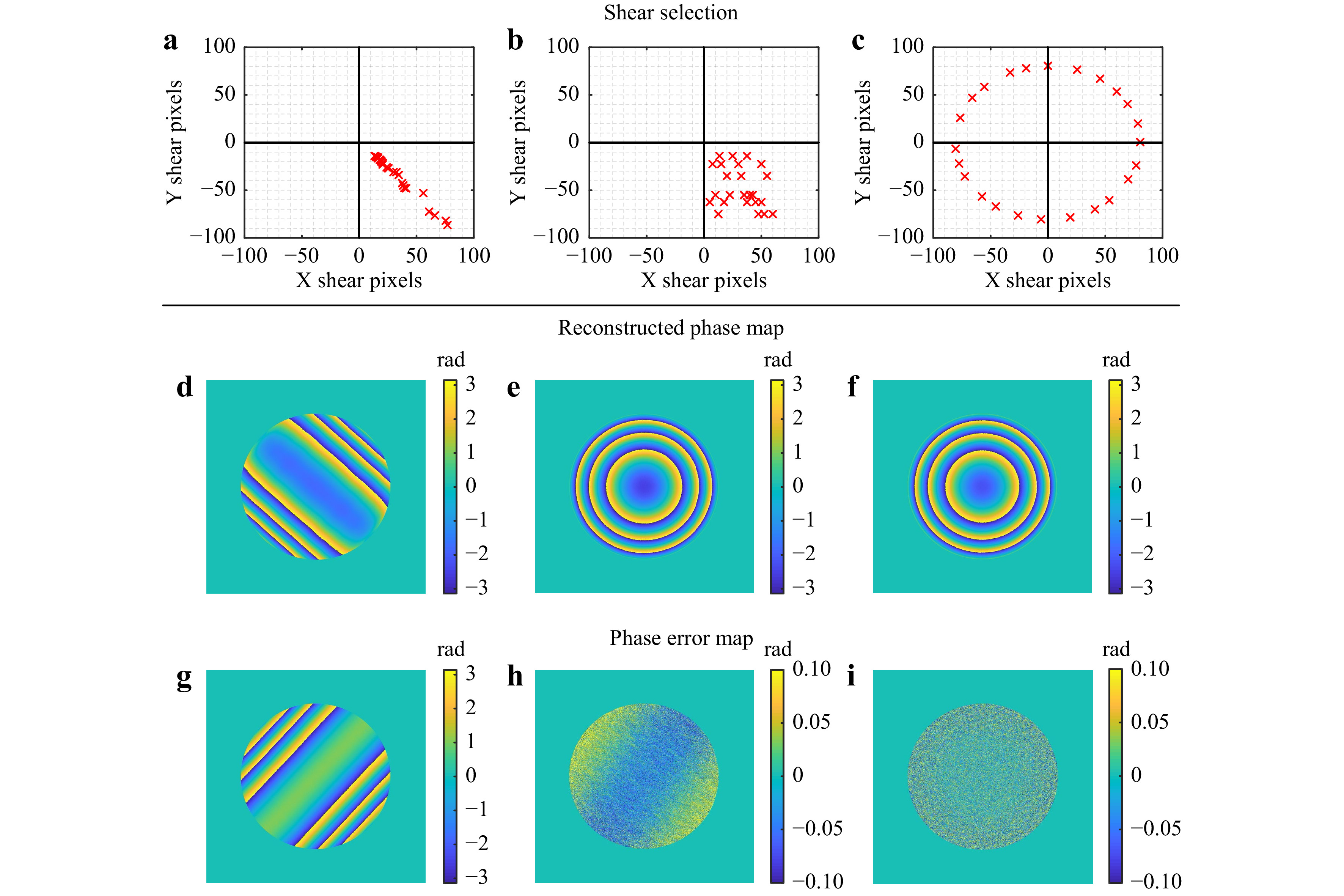
Fig. 10  Comparison of reconstruction results between different configurations. a Shear selection for test 1 in cartesian coordinate configaration. b Shear selection for test 2 in cartesian coordinate configuration. c Shear selection for polar coordinate configuration. d Reconstructed phase map from test 1. e Reconstructed phase map from test 2. f Reconstructed phase map from polar coordinate configuration. g Phase error map from reconstruction using test 1 parameters. h Phase error map from reconstruction using test 2 parameters. i Phase error map from reconstruction using polar coordinate configuration.

Each simulation was performed with 24 shears, where the selections are shown in Figs. 10a−c. The selections analyze two possible xy-shearing configurations shown in Fig. 10a, b (see Fig. 2 for configuration) and the fixed shear with variable shear axis shown in Fig. 10c (see Fig. 3 for configuration).

In test 1 (Fig. 10a), the shears have been selected along an approximately linear trend. The reconstructed phase map from this shear selection showed that some of the frequencies were not being reconstructed correctly, which is a consequence of the ambiguity that arises from the measured data. The reconstruction results are shown in Fig. 10d, g. When the selection of shears was scattered across one quadrant (Fig. 10b) as in test 2, the reconstruction algorithm had sufficient data to reconstruct most of the point-source wavefield, as shown in Fig. 10e. However, the error map in Fig. 10h shows a curvature, indicating the possibility of some missing frequencies. This slowly varying error is critical as it produces a so-called form error that is difficult to filter out when observing aperture size measurement objects (e.g., mirrors or lenses under test). This error may be less critical when the sample is small (e.g., in the case of a cell under a microscope). The shear selection shown in Fig. 10c is based on a variable shearing axis but with a fixed shear amount. The latter system allows accessing all four quadrants, and the shears can be selected at all possible rotation angles of the shear axis. The reconstruction is shown in Fig. 10f. The error map shown in Fig. 10i shows that the error map is dominated only by high-frequency noise patterns, which can be filtered more easily. These results demonstrate that selecting shears across all quadrants results in better reconstruction because it provides more information for a successful reconstruction.

To better understand the results and characteristics features in the error maps of Fig. 10, further study was done using transfer function analysis to investigate the effectiveness of the selected shear sets to transmit information for wavefield reconstruction. Extensive studies have been done by Falldorf ²⁵ for non-symmetric shears and Servin²² for symmetric shears in understanding the frequency response of spatially shearing systems. Inspired by Servin’s description²² for the transfer function, we define the frequency information density as

where $ \overrightarrow{k}=\left[{k}_{x},{k}_{y}\right] $ is the frequency coordinate and $ \overrightarrow{ds}=[d{s}_{x}, $$ d{s}_{y}] $ is the shear in x- and y- directions. This transfer function analysis estimates the “frequency information density” at each spatial frequency coordinate for a given set of shears. These functions were evaluated and mapped for all three configurations as shown in Fig. 11.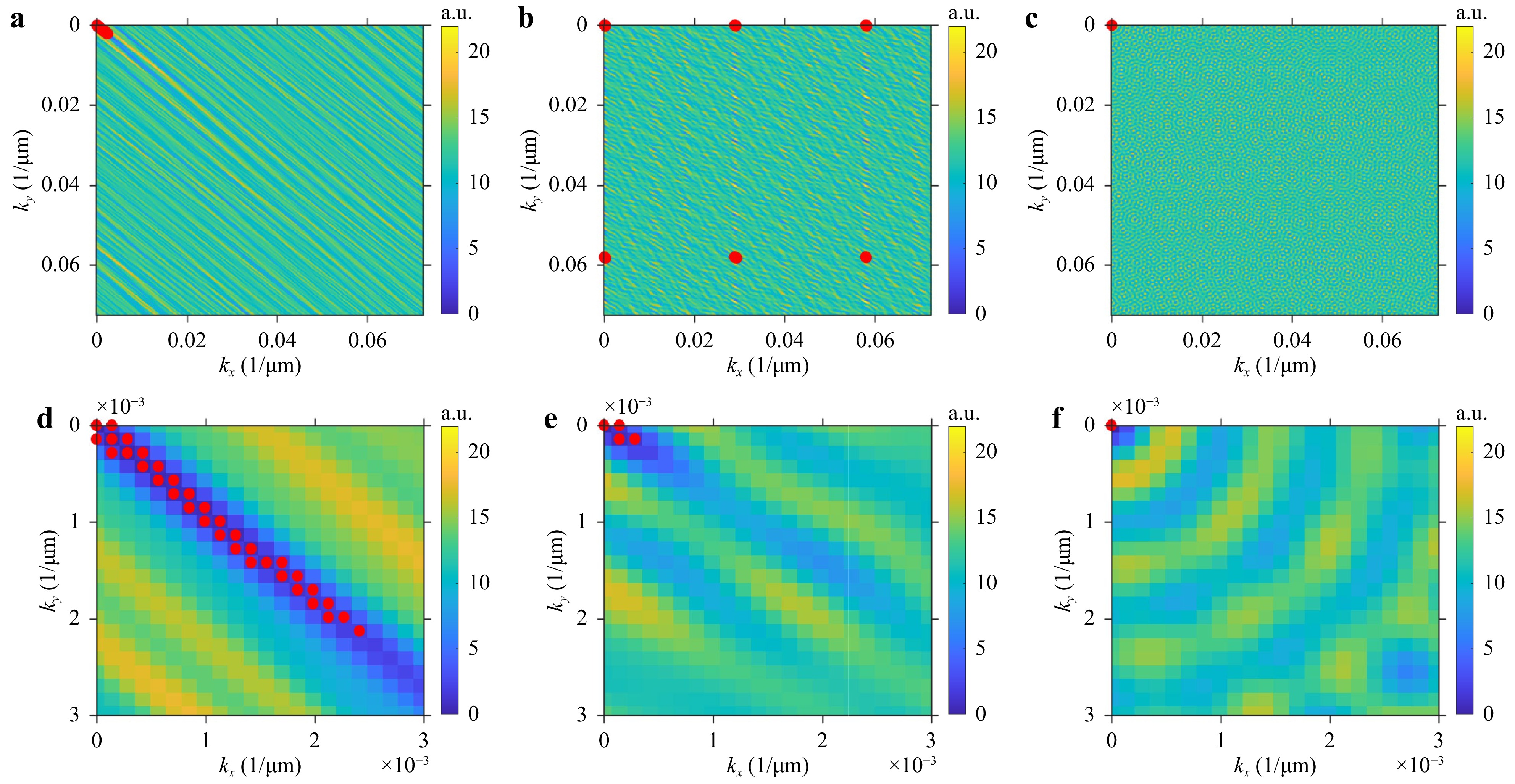

Fig. 11  Transfer function analysis (Frequency information density plots with points below threshold 2): a Test lin cartesian coordinate configuration (34 datapoints below threshold). b Test 2 in cartesian coordinate configuration (21 datapoints below threshold). c Polar coordinate configuration (1 datapoint below threshold). d Test 1 plot in cartesian coordinate configuration zoomed near small frequency regions. e Test 2 plot in cartesian coordinate configuration zoomed near small frequency regions. f Polar coordinate configuration plot zoomed near small frequency regions.

Figs. 11a−c are the frequency domain information density maps for the three shear sets described in Fig. 10. Figs. 11d−f are the same maps but zoomed in near low spatial frequencies to visualize better the behavior at these regions, where regions below the threshold of 2 are highlighted in red. Fig. 11d shows a significantly high amount of frequency sets that have transfer function values below the threshold. These cluster appear to dominate in regions where kx ≈ ky. This indicates that a large number of frequencies along the 45-degree angle will have poor reconstruction in the estimated wavefield at longer spatial wavelengths. This conclusion is in agreement with Fig. 10g. A similar behavior is observed in Fig. 11b, e, however, the number of frequency sets with transfer function values below the threshold of 2 are located at both low and high frequencies, with a minimal presence near low spatial frequencies. The locations of these cluster indicate that very low spatial frequencies will appear in the error map but will have better reconstruction than the previous shear set. This is observed in Fig. 10h, but there are also high frequency errors present due to low values of the transfer function at higher spatial frequencies. The polar configuration in Fig. 11f has no transfer function values below the threshold of 2, except for the (trivial) frequency at (0,0). This indicates good reconstruction of the estimated wavefield at all spatial frequencies.

The following section demonstrates how spatial overlaps between different shears impact the reconstruction of the final wavefield. When an object wavefield passes through the gratings, it splits in two, represented as beam 1 and 2 in Fig. 12a. Depending on the shear amount, there is an overlap region between the two beams (overlap region is indicated in yellow). Since the overlap region produces an interference pattern, the phase information from the overlap region feeds into the algorithm. Fig. 12b shows which areas of the input beam provide phase information to the reconstruction algorithm (regions indicated in yellow).

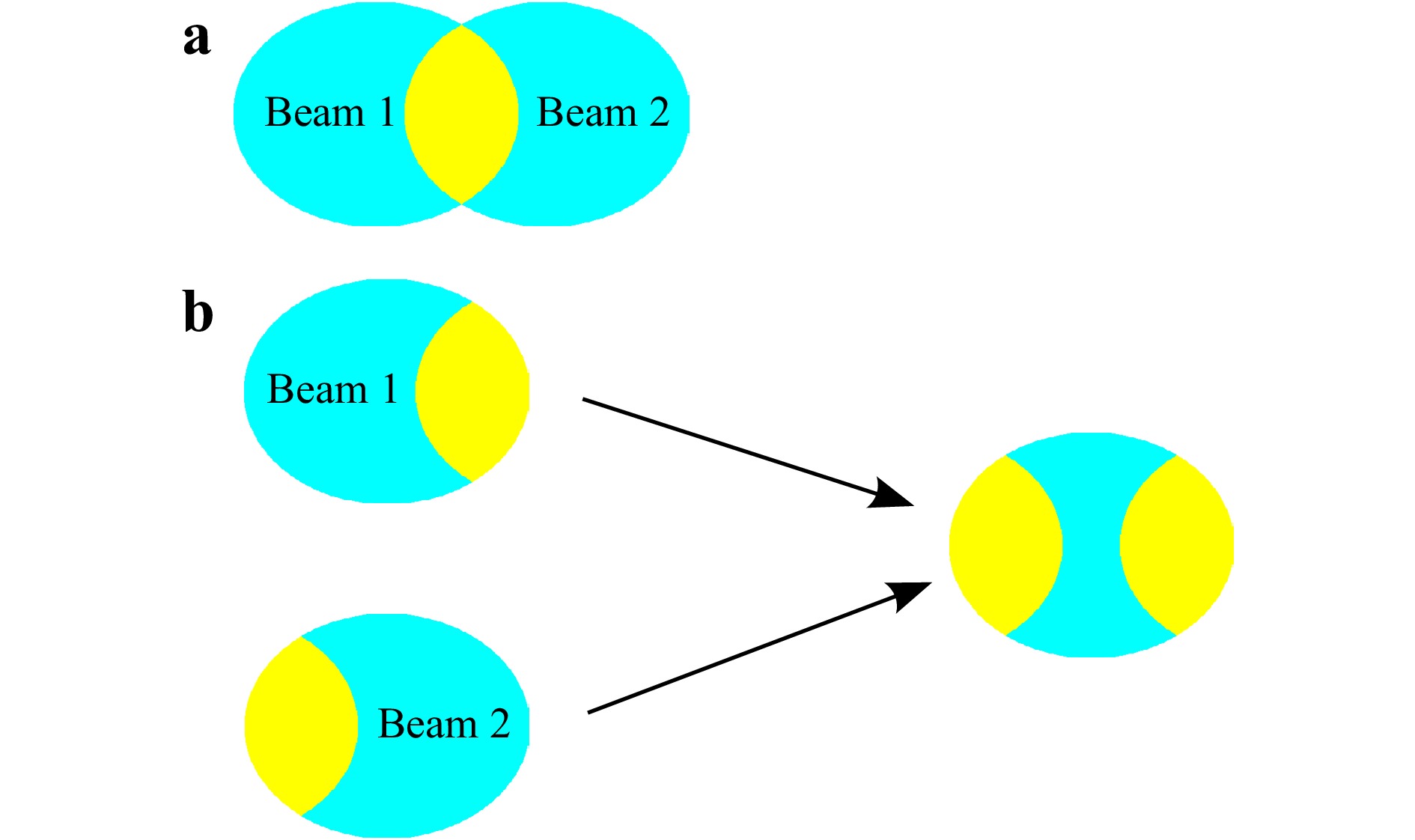
Fig. 12  Demonstration of data recorded by each shear: a Beam 1 and 2 overlapping. b Summation of overlapped regions indicating regions that have data for reconstruction (yellow regions).

This idea is further extended to multi-shear interferometry in Fig. 13. Fig. 13a shows the overlap regions from an object beam with a diameter of 600 pixels sheared by 175 pixels along the x-direction. Fig. 13b shows the overlap regions if a second shear is added to the measurement in the orthogonal direction by the same amount. In Fig. 13b the yellow areas indicate regions with two overlaps, green areas indicate regions with one overlap, and the dark blue areas indicate regions with no overlap. This idea is extended over 24 shears in Fig. 13c, showing a significantly higher count of overlaps (or number of effective measurements). This case also shows an example of a situation where the algorithm will not completely reconstruct all spatial frequencies near the wavefront’s center because the chosen fixed shear is too large (175 pixels). Fig. 13d shows an alternative set of 24 shears (i.e., with a small shear amount compared to (c) with 80.5pixels). There, all of the spatial locations have been measured at least 20 times. The case presented in Fig. 13d has the highest potential to successfully reconstruct the wavefield due to maximum overlap across the whole area.

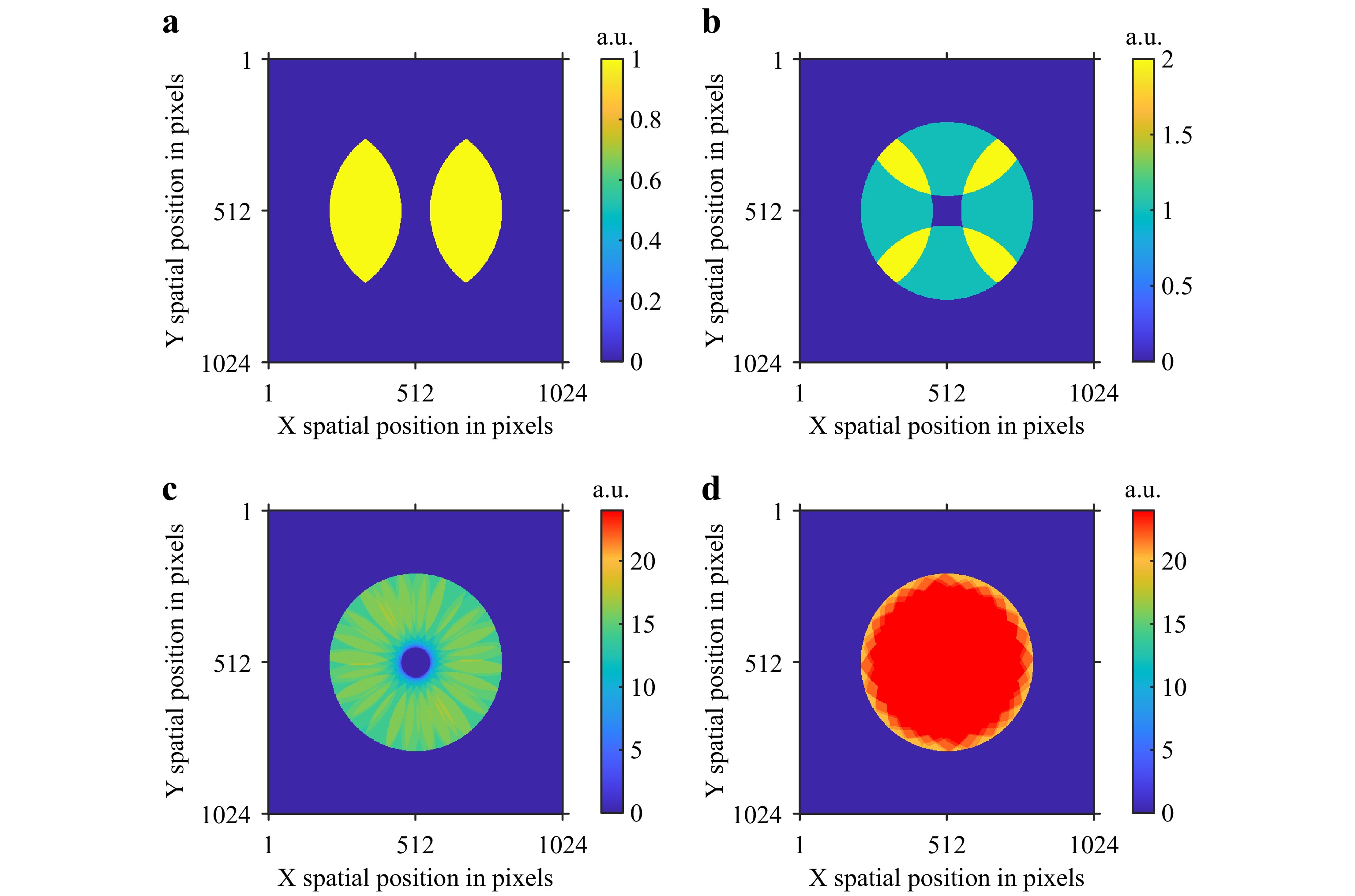
Fig. 13  Spatial information density distribution for different shear patterns on 1024 × 1024 pixel maps with aperture diameter of 600 pixels. a Single shear of 175 pixels. b Two orthogonal and equal shears of 175 pixels. c 24 shear in polar configuration with a fixed shear of 175 pixels. d 24 shear in polar configuration with a fixed shear of 80.5 pixels.

It should be noted that (as discussed by Servin²²) the wavefront may be reconstructed even at regions where there is no overlap. This phenomenon is especially true for lower spatial frequencies because they do not need to be sampled everywhere. However, the reconstruction is increasingly difficult at higher spatial frequencies at a given location if no interference exists.

The same concept is applied to the three configurations / shear sets discussed in Fig. 10 and the overlap distribution is mapped in Fig. 14. Fig. 14a, b show fewer overlaps along the boundary at 45-degree angle. The number of effective measurements drops from 24 to 13. On the contrary, Fig. 14c shows uniform distribution of overlaps covering the majority area of the object beam. At the border, there are still 20 effective measurements recorded, which indicates better reconstruction across the whole area of the object.

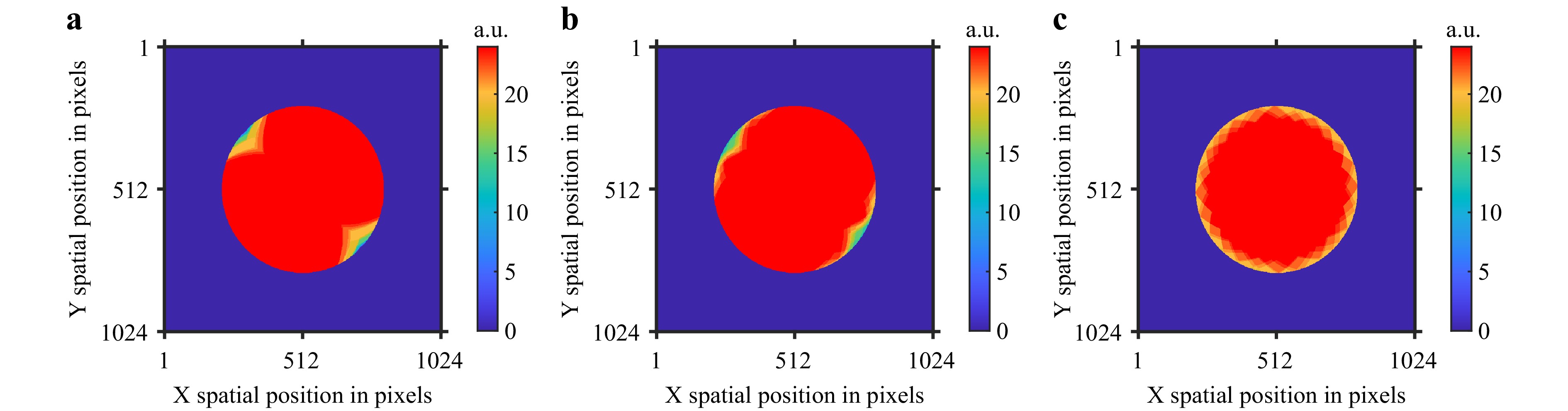
Fig. 14  Spatial information density distribution across all three configurations with 24 shears. a Test 1 in cartesian coordinate system (linear pattern). b Test 2 in cartesian coordinate (shears in scattered pattern). c Polar coordinate system with shears at unequal angles.

Any error present in the estimated shear value propagate through the reconstruction process and result in an error in the final reconstructed wavefield. This mismatch between actual and assumed shear amounts can result in error artifacts in the reconstructed wavefield or missing frequencies from the original wavefield. Monte-Carlo simulations were carried out to evaluate the effect of errors in the estimated shear pixels in reconstructing the wavefield by adding normal distributed random errors to the shear values in X and Y direction for the shear configuration in Fig. 10c (100 simulations for each case). Furthermore, a total of 20% intensity noise (of the peak value) has been added to all interferograms to include the effects of noise in realistic measurement conditions.

This series of simulations provides an overview of how the phase errors in reconstructed wavefields are affected by the imperfect shears. The results of the series of simulations have been summarized in a box plot, as shown in Fig. 15. As expected, when observing the RMS error in the reconstructed phase, there is a clear correlation with the increasing amount of shear error. However, it is interesting to notice that the different spatial frequencies are affected in different ways; as the standard deviation of the shear error increases, the ability of the algorithm to reconstruct higher spatial frequencies decreases. Figs. 15b−d show the measurement of a USAF target where the Monte Carlo simulation used a shear error of 1-, 3-, and 5-pixels standard deviation, respectively.

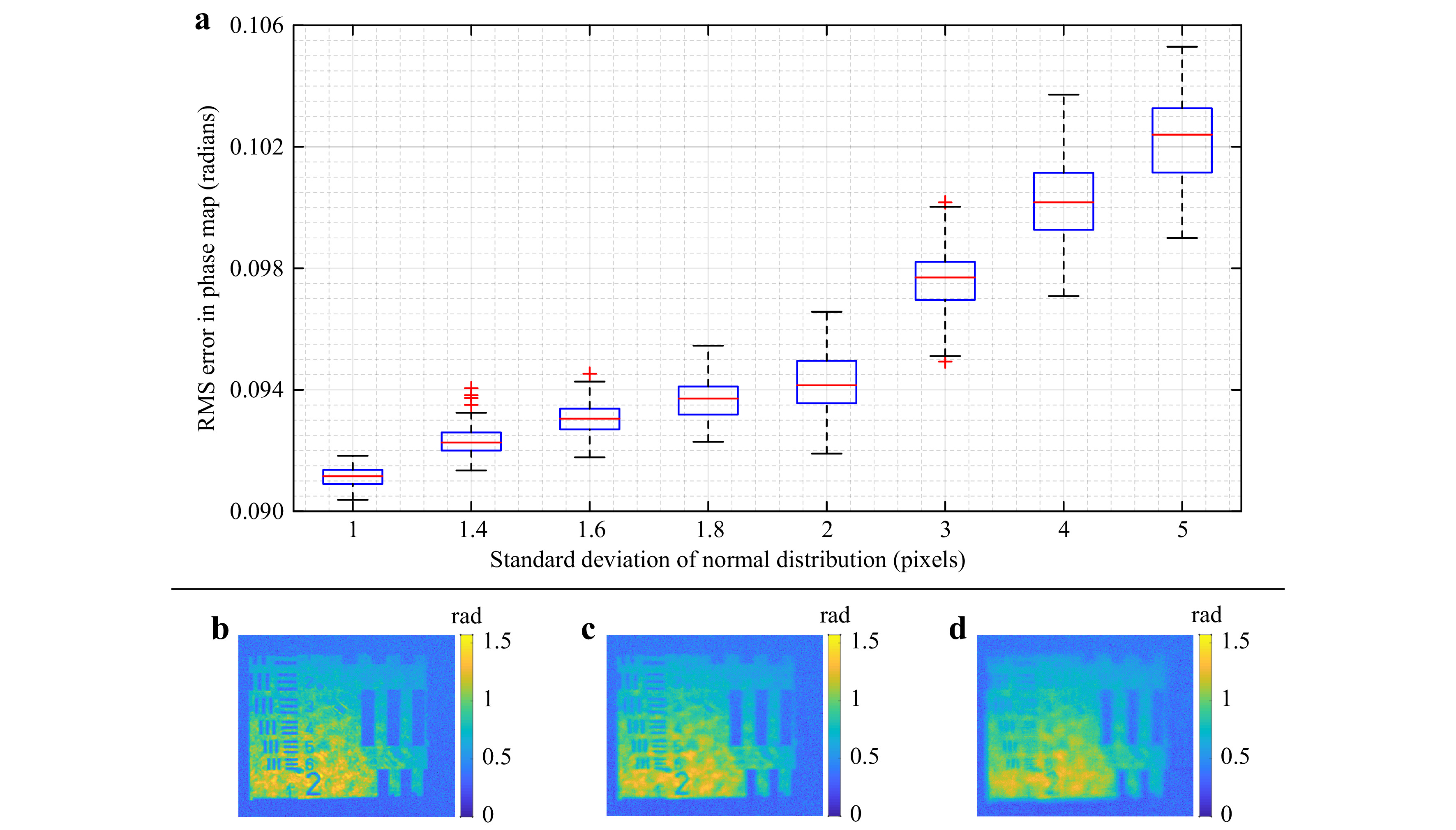
Fig. 15  a Box-plot showing a summary of the simulations. b Reconstructed phase map at standard deviation 1 pixel. c Reconstructed phase map at standard deviation 3 pixels. d Reconstructed phase map at standard deviation 5 pixels.

The reconstruction algorithm requires the shear amount to be known. As concluded from the Monte Carlo simulations, the better the estimation of the shear amount, the lower the reconstruction error and the higher the spatial resolution. In this work, we have estimated the shear amount by calculating the auto-correlation of the recorded intensity maps. To increase the robustness of this estimation, we have removed the sinusoidal fringe modulation by averaging all four measured phase-shifted intensity patterns. One examplary measurement is shown in Fig. 16a. The second-order derivative of the auto-correlation map has been computed along one direction to further enhance the peak in the auto-correlation map. The resulting spikes for the case in Fig. 16a are shown in Fig. 16b, and they are prominently identifiable. The second-order derivative of the auto-correlation map comprises three peaks: a center peak and a peak on either side of the center peak, which is located at twice the value of the actual positive and negative shear amounts. The shear amount is estimated by tracking one of the side peak positions to the center peak. The difference in X and Y coordinates of the side and center peak gives twice the shear value for each averaged intensity map. The actual shear can be detected down to an accuracy of 0.5 pixels.

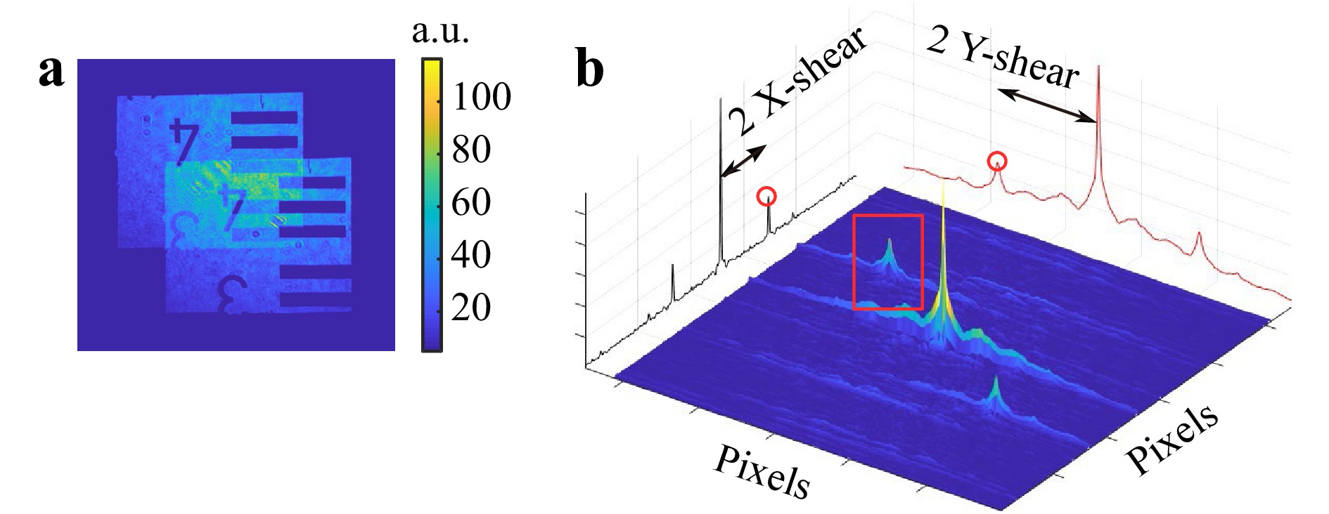
Fig. 16  a Intensity map with sheared images of object. b Second derivative of auto-correlation map showing peaks corresponding to shear in X and Y direction.

When working with left and right circular polarized waves, it is convenient to employ pixelated polarization cameras to record four phase-shifted intensities simultaneously. The polarization camera enables single-shot phase-shifting during the measurement process for each shear. The single-shot phase-shifting capability offers an advantage in reducing the number of translation axes, enhanced stability, and mitigation of alignment errors. The reduction of the number of translation axes further ensures repeatability.

Commonly, each super-pixel on the detector of the polarization camera has four pixels that record the image at four different polarizer angles. As the two incident waves have a left-circular and right-circular polarization, it is possible to obtain simultaneously four interferograms at four different phase shifts. The orientation of this pixelated array is shown in Fig. 17, which also shows an example of a defocused point source measured at a single fixed shear with 0°, 90°, 180°, and 270° phase shifts. The recorded intensities have a resolution of 1024 × 1024 pixels.

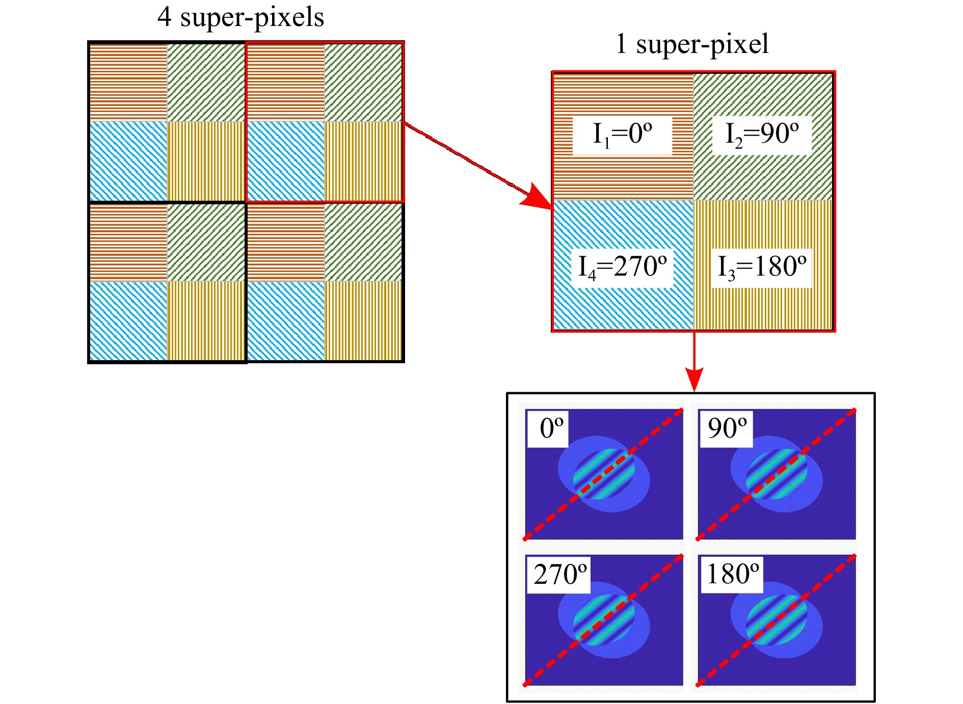
Fig. 17  Schematic of the polarization camera sensor and intensity maps demonstrating the phase shifts.

One critical correction is needed before the phase can be calculated. The individual frames are often clustered in a super-pixel and can be separated without difficulty. However, all four frames are not located at the same spatial position. An additional interpolation is needed (e.g., including the Fourier shift theorem) to obtain all four interferograms at the same spatial location. In this work, we have compensated this spatial mismatch for the interferograms I2, I3, and I4 (but not I1), to obtain an interferogram that is shifted by 1/2 super-pixels.

Fig. 18 shows the experimental setup for the Cartesian coordinate shear setup, along with a schematic showing the arrangement of optical components for the setup. The light source illuminating the object is a class 3B, 520 nm wavelength, 30 mW green laser. The object used for the experiments is a USAF target. Two sets of lenses with 4f configuration were used to keep the aperture 1 and the object in focus. Aperture 2 was used to limit the effects of stray light, back reflections, and the higher-order diffraction orders. A polarization camera was used to capture the four phase-shifted interferograms simultaneously (FLIR Blackfly-S model BFS-U3-51S5P-C). The grating arrangement is shown in detail in Fig. 19.

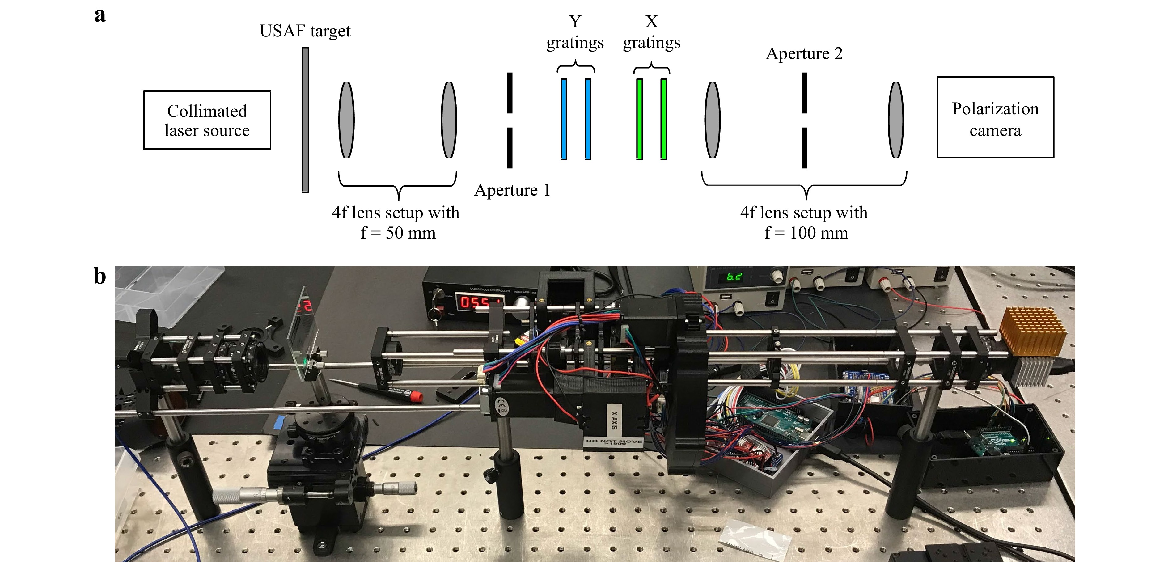
Fig. 18  Experimental setup for Cartesian coordinate shear setup a schematic b experiment.

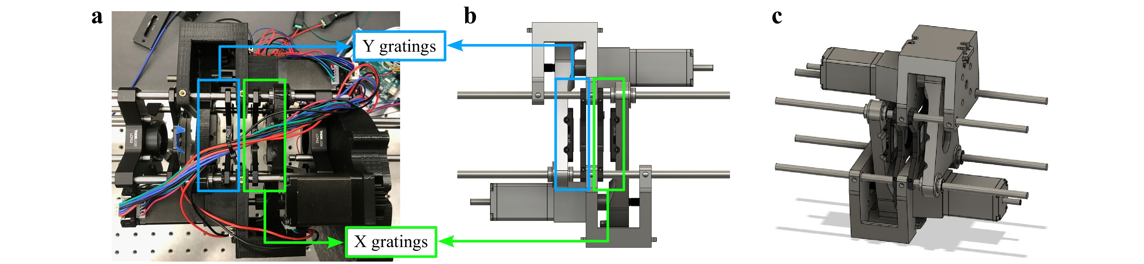
Fig. 19  Grating arrangement in Cartesian coordinate shear setup a experimental setup b schematic of the setup c 3D schematic of the setup.

The cartesian coordinate shear system in Fig. 19a has four polarization gratings, two on the left-hand side (blue) to shear the wavefield in the vertical direction (y-direction), and the two on the right-hand side (green) to shear the wavefield in the horizontal direction (x-direction). Two leadscrew stages are connected to the two outermost X and Y polarization gratings which translate along the Z-axis to create the shears. The leadscrew stages utilize stepper motors and encoders to accurately determine the stages' position and limit switches for homing the system. Additive manufacturing (3D printing) was used to construct the stage, and accompanying electrical circuitry and software were developed for the closed-loop control system. The two inner gratings are fixed. Since only one grating can move in each grating pair, the shears are limited to only one quadrant (see Fig. 10a, b).

An experiment was carried out to validate the previous findings regarding the shear configuration in Fig. 10a. The results for the first configuration are shown in Fig. 20, where a total of 24 different shear amounts have been applied (see Fig. 20a) using an instrument that can independently adjust the x- and y- shears. The object used in this experiment is a simple section of an amplitude USAF target, where the remaining sections are blacked out due to aperture 1 (see Fig. 18a).

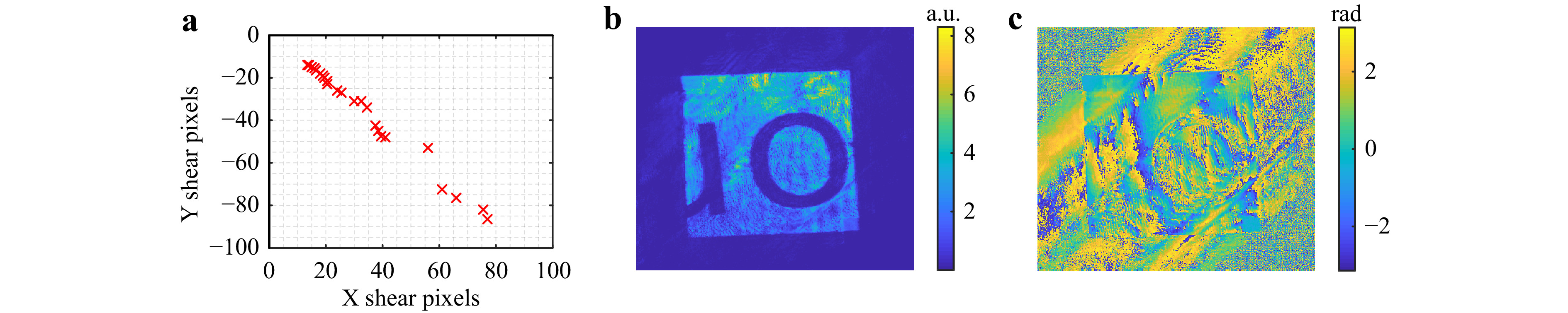
Fig. 20  Reconstructed results from cartesian coordinate shear experiment a shear selection b amplitude map c phase map.

The shears were estimated from experimental data using the auto-correlation method, as discussed in the previous section. Once the shears were estimated, they were given as input to the algorithm to reconstruct the wavefield. A multi-resolution technique¹⁰ was implemented within the reconstruction algorithm to mitigate the effects of initial guesses and improve the convergence. For our dataset with 1024 × 1024 pixels, a 5-level multi-resolution reconstruction starting from the coarsest grid with 64 × 64 pixels was implemented. The estimated wavefield is then up-sampled by a factor of 2, and the reconstruction process happens at a higher resolution (i.e., 128 × 128 pixels) using the newly up-sampled wavefield as the initial guess. This process repeats until the estimated wavefield reaches the original resolution, i.e., 1024 × 1024 pixels. The results for this 5-layer multi-resolution approach are shown in Fig. 20.

The reconstructed amplitude map (Fig. 20b) shows the object features that would be expected. However, the phase map in Fig. 20c shows the presence of parasitic signals. This reconstruction is expected given the outcome of previous simulations, see Fig. 10. This is a direct consequence of the shear selection: most of the shears selected for this experiment are dominant along the -45° angle. This selection has generated parasitic signals along the 45° angle, as seen in Fig. 20c.

The other shear configuration that produced consistently better results was the configuration of a fixed shear with a variable shear axis, see Fig. 10c. An experimental implementation is shown in Fig. 21, where the xy-shear system in Fig. 18 is replaced with a simple two grating set up on a rotational mount. Fig. 22 shows a more detailed view of the shearing mechanism. Notably, the 2-grating setup can be realized in a more compact optical setup; however, we chose to keep the 4f configuration to compare the two setups better. The results for the configuration in Fig. 21, using 24 different shear amounts, are shown in Fig. 23. Similar to the case of Fig. 20, a portion of the USAF target has been selected for the measurement, and the field of view is limited by aperture 1 (see Fig. 21).

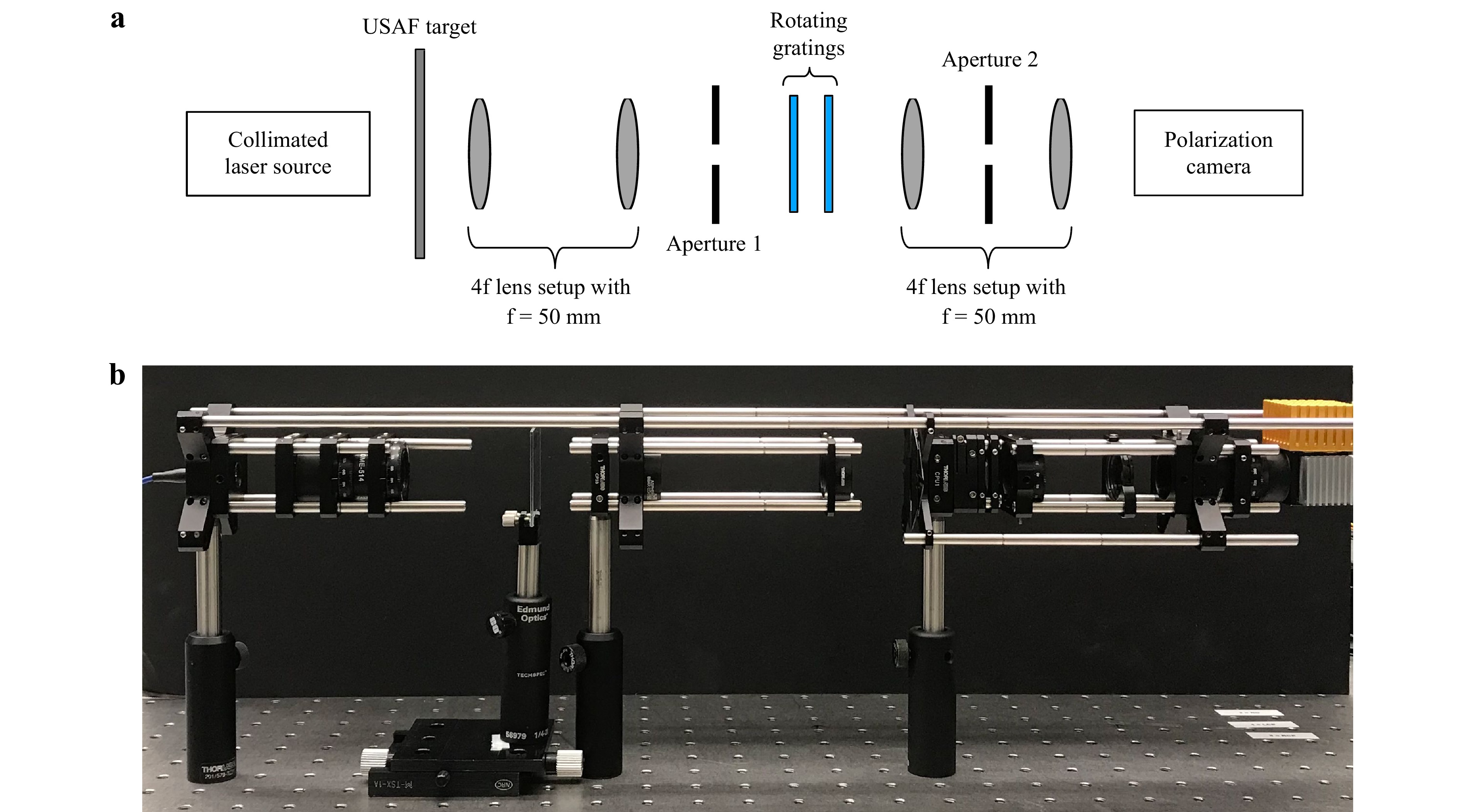
Fig. 21  Experimental setup for polar coordinate shear system a schematic, b experiment.

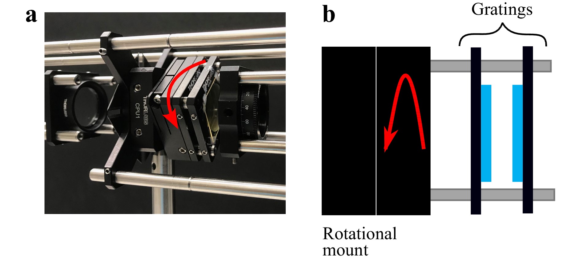
Fig. 22  Gratings arrangement in polar coordinate shear configuration a Experimental setup showing the rotation of gratings. b Schematic of the grating arrangement.

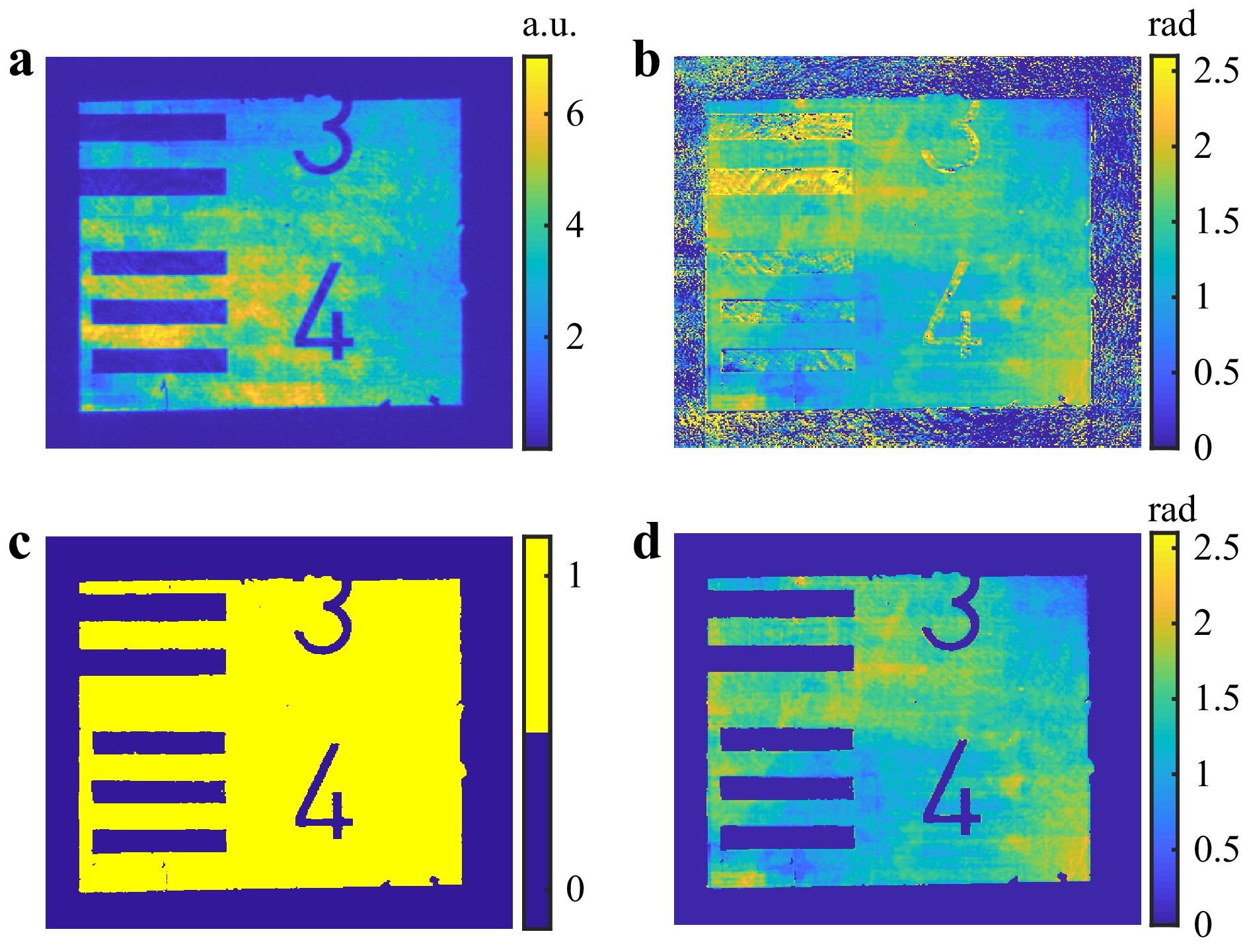
Fig. 23  Reconstructed results a amplitude map b phase map c mask from amplitude map d phase map with mask applied.

Fig. 23a, b show that the solver successfully reconstructs both the amplitude and the phase map, free of parasitic fringes. For better visualization, a mask has been generated (see Fig. 23c) using the amplitude information and applied to the phase data (see Fig. 23d).

A further experiment has been conducted to verify that the instrument in Fig. 21 can capture and reconstruct the wavefield at a defocused distance. For this purpose, we shift the camera's position by a distance of ~170 mm, so that both the object and the aperture get defocused by the same amount.

The reconstructed wavefield is shown in Fig. 24a, c. After reconstruction, the wavefield was numerically refocused to the visually best reconstruction distance (z=162.94 mm) using the Angular Spectrum method^26,27. The results of the refocused wavefield are shown in Fig. 24b, d. For better visualization, various regions of the reconstructions have been zoomed in and are presented in Fig. 25.

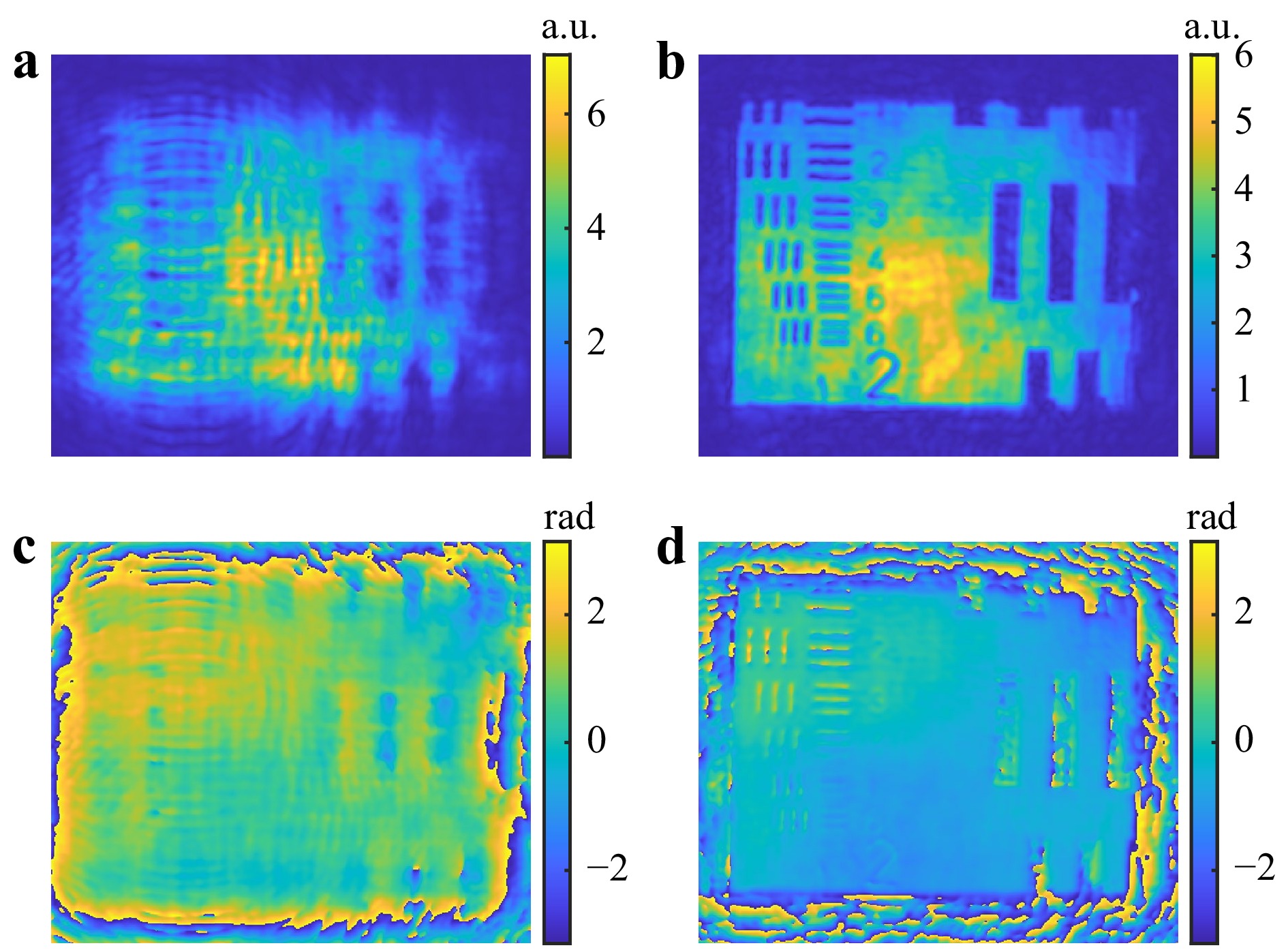
Fig. 24  Reconstructed results from defocused object a amplitude map before numerical refocusing. b Amplitude map after numerical refocusing. c Phase map before numerical refocusing. d Phase map after numerical refocusing.

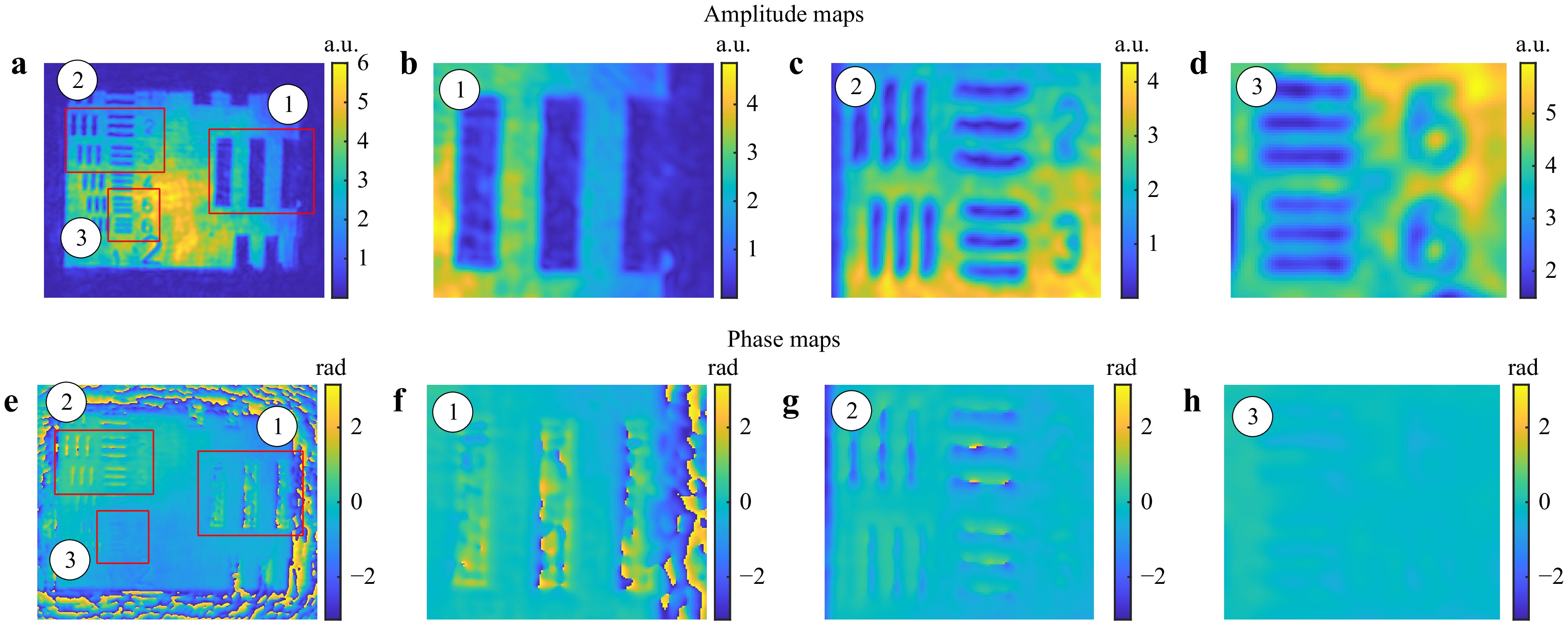
Fig. 25  Reconstructed wavefield of defocused object (zoomed) after post processing: a Amplitude map of the full object. b Region 1 amplitude map. c Regions 2 amplitude map. d Regions 3 amplitude map. e Phase map of the full object. f Region 1 phase map. g Region 2 phase map. h Region 3 phase map.

The light source used for the experiment is an FC-520-040-PM laser system (520 nm, 30 mW) from CivilLaser. The object sample is a combined USAF 1951 and Dot Grid Target (Edmund Optics #62-465). The GP gratings have been purchased from Edmund Optics (#12-677, 96% diffraction efficiency at 550nm, 159grooves/mm, 25 × 25 × 0.45 mm). The light illuminating the object is linearly polarized to produce 50% RHCP and 50% LHCP at the GP grating, maximizing the fringe visibility. The camera used for imaging is a FLIR Blackfly-S model BFS-U3-51S5P-C polarization camera. The lenses used for the 4f-configuration have an effective focal length of 50 mm.

In this work, a GP grating-based shearing holography system has been presented. The GP gratings used in this work have the unique ability to have a polarization-sensitive diffraction angle, where the RHCP and LHCP light beams are diffracted in two different directions. Figs. 1−3 show how these properties can be exploited with a linear polarizer to create an adjustable shearing interferometer. This paper presented two distinct configurations, (i) one that allows for adjustable xy-shearing, and (ii) one that keeps the shear amount constant but rotates the shear axis. Another aspect of the GP grating-based shearing interferometer is that a series of phase-shifted interferograms can be obtained by either rotating the polarizer (see Fig. 4) or using a pixelated polarization camera (see Fig. 17).

The ability to produce a series of phase-shifted interferograms obtained under various shear amounts opens the possibility to obtain high fidelity data that can be processed in a wavefront reconstruction algorithm. In this work, we have implemented the approach of Konijnenberg¹⁶ outlined in Fig. 5 but added a filtering procedure to remove algorithm-specific artifacts (see Fig. 6d, Figs. 7−9). We further investigated the effect of the shear selection. Fig. 10 showed that choosing the shears to be on a circle in the sx-sy plane provides consistently good results, where the error is of high-frequency nature. These findings are supported using Servin’s²² transfer function analysis and spatial domain support that were referred to as “frequency domain information density” (see Fig. 11) and “spatial domain information density” (see Fig. 14). One critical step is the estimation of the exact shear amount. Any discrepancy between the actual shear amount and the values used within the wavefront reconstruction algorithms will increase, to some degree, the RMS in the reconstructed phase, see Fig. 15. However, the results in Fig. 15 also show that an imperfect shear estimate value has a strong impact on the resolution of the reconstructed wavefield (even if the RMS increases only marginally by 10%, for the case of typical levels of intensity noise). To ensure accurate results, we have reported a shear estimation technique using the second derivative of the autocorrelation function, where the spikes of that function estimate shear amount down to an accuracy of 0.5 pixels, as shown in Fig. 16. The reconstruction algorithm presented in this paper does not limit the possible applied shears. The algorithm can process sub-pixel shearing as the algorithm primarily operates on FFTs. However, the shear detection technique presented in this paper is limited in identifying shears. The procedure detects twice the values of shears for a sheared interferogram as integer, and hence the shears can be estimated down to integer multiples of 0.5 pixels. More sophisticated shear detection algorithms (using weighted mass algorithms or techniques based on ideas from Guizar-Sicairos M. et al²⁸.) might enable finer shearing detection down to 0.01 pixels and are subject to future research.

The previous aspects have been verified experimentally for both shearing configurations, as shown in Fig. 18,19 for the xy-shearing component and Fig. 21,22 for the configuration that rotates the shear axis. As expected, the system configuration that keeps both gratings fixed while the grating pair rotates about the optical axis provides the visually best reconstruction result with no parasitic fringes, as shown in Fig. 20,23. A further advantage of the setup with the variable shear axis is that it requires only two GP gratings and can be, in principle, incorporated into a more compact setup. There are also several motorized rotating mounts available that could automate this process.

Finally, we demonstrate the feasibility of this approach by reconstructing the wavefield of a defocused object at the distance z = 162.94 mm. Refocusing using the Angular Spectrum method^26,27 produces Fig. 24,25.

These findings show the advantage of GP grating-based shear interferometers compared to conventional dual grating (or dual double-grating) configurations. A conventional dual-axis grating-based variable shearing interferometer with phase shift capabilities requires two independent axial shifts of the x- and y- gratings (to adjust the shear) and lateral shifts of the gratings in x- and y- direction (for phase-shifting). Having to control four mechanical axes independently is a significant system complexity, where the freedom to adjust all parameters appropriately is often compromised due to space constraints. In contrast, the results of this work show that a GP grating configuration with a fixed shear amount, but an adjustable rotational shear axis can provide the shear selections for robust measurements while maintaining phase-shifting capabilities using a pixelated polarization camera. In other words, robust variable shearing interferometry can be made possible by controlling only one mechanical axis (instead of four). This finding has implications for future compact interferometer designs.

The authors acknowledge the support and funding from the Center for Precision Metrology (CPM).