Reflections about the holographic and non-holographic acquisition of surface topography: where are the limits?

For the first-ever observers of a holographic recording at the 1964 OSA spring meeting¹, the most intriguing feature was probably the three-dimensional appearance of the reconstructed object. After 60 years of holography, this ‘magical’ effect still captivates observers who can freely change the viewing perspective and locally focus on the object’s surface. The reconstruction seems to be perfect, indistinguishable from the true object, including phase and amplitude. Holography is based on the interferometric superposition of waves, which suggests ultraprecise measurement options, and indeed, holographic interferometry is a paradigm for this option², as well as the holographic Null test³ via computer-generated holograms, invented by Adolf Lohmann⁴. Holographic microscopy flourishes with the availability of high-resolution camera chips⁵⁻⁷. A hologram records a complex field, sometimes called a “wavefront”, originating from an object under test. This field can be read out optically or computationally. For a proper source encoding, we can modify the recording by placing some optical instrument in front of the holographic plate, e.g., a shearing plate. Furthermore, we can place any optical instrument behind the (analog) hologram to extract specific information about the object. With a camera chip replacing the holographic film, any instruments and much more can be mimicked via computation.

This article discusses the potential and limits of measuring the surface shape or topography, meaning the spatially resolved distance $ z(x,y) $. We investigate holography and its major competitors regarding what is similar and different. The topographical information can be deciphered by numerous methods discussed below. We aim to know the physical source of the dominant noise that ultimately limits the achievable uncertainty of measurement, in other words, the lowest possible statistical distance uncertainty $ \delta z $.

It will be discussed how holographic methods compare to the established non-holographic methods. Some methods have a close connection to holography; for others, the connection is only indirect. We will look at the problem from a bird’s eye view. More details and further references can be found in⁸. The idea of exploiting physical limits to advance optical 3D metrology is described in [9]. From the knowledge of the limits, the user may find out if his measurement results could be improved (for example) by better hardware - or if the results are already hitting the ultimate physical limit. The considerations will also help the manufacturer of 3D metrology find out if the competitor can really and truly satisfy the advertised specifications or if there might be some exaggeration.

We summarize our considerations:

● What is the physical origin of the ultimate measuring uncertainty?

● How is the topography encoded and decoded?

These questions are useful to bring some order into the overabundance of available 3D sensors and help customers understand the limits and the potentials of different sensor principles. Our questions intentionally avoid hardware aspects and solely consider fundamental physical principles.

Optical sensors exploit different kinds of illumination, such as coherent/incoherent, structured/homogeneous, monochromatic/colored, polarized/unpolarized... There are different ways of interaction with the object surface: coherent (Rayleigh scattering), incoherent (thermal, fluorescent), specular/diffuse, surface/volume... The detected modality may be the intensity, the complex amplitude, time-of-flight, polarization, coherence. Permuting all those parameters leads to more than 10,000 possible sensors. Not all of them are physically different, but there are differences significant for the user of 3D sensors. Surprisingly, it turns out that all sensors (so far considered by the authors) belong to only four different measuring principles, which can be classified by the physical origin of the fundamental distance uncertainty. An important parameter for users is the dependence of the distance uncertainty (not the accuracy and lateral resolution) on the aperture (we refer to earlier investigations⁸). The results are condensed in Table 1. The competing measuring principles (see as well Fig. 1) are triangulation (I), classical interferometry (II), rough-surface interferometry (III). There is a category IV that we name “slope-measuring methods”. This class comprises methods that intrinsically measure the surface slope or lateral derivative. Table 1 summarizes the fundamental distinction between the categories or classes and displays the recipes to calculate the corresponding limits. Fig. 2 illustrates the systems theoretical simiilarity of hlography with fringe projection triangulation. Fig. 3 displays coherent noise which is the ultimate uncertainty limit of triangulation systems. Figs. 4, 5 illustrate that different measuring principles (here III and IV) display very different limits of the uncertainty of measurement.

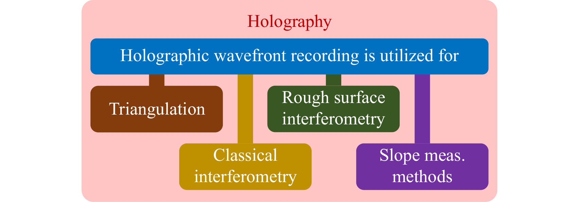
Fig. 1  Holographic acquisition of surface topography: The outstanding feature to record an optical wavefront in a hologram can be utilized in many different ways to measure the surface topography of an object. Respective measurement principles can be categorized into four groups: triangulation, classical interferometry, rough surface interferometry, and slope measuring methods.

In the following, we give a few examples for each class: Amongst others, class I (triangulation) comprises laser triangulation, stereo-photogrammetry, focus search, fringe projection triangulation, or structured illumination microscopy. We note that the wide area of fluorescence methods is not discussed here. Class II (classical interferometry) comprises essentially interferometry at specular surfaces. Whether a surface is ‘optically specular’ or ‘optically rough’ depends on the surface and on the observer: specular means that the local topography $ z(x,y) $ within the optically resolved area (the diffraction disc) varies less (or better much less) in depth than a quarter of the used wavelength to avoid destructive interference and speckles. For a specular surface, the complex signal degenerates to $ exp(ikz) \approx 1+ i kz(x,y) $, with the consequence that the coherent lateral averaging over the diffraction disc leads to a signal corresponding to the mean distance $ {<z(x,y)>} $. For optically rough objects (i.e., for large height variations within the diffraction disc), however, the term $ <exp(ikz(x,y))> $ is a nonlinear and non-monotonic (‘chaotic’) function of z, leading to the typical random walk of the complex signal and speckle. In class III, we find rough-surface interferometry which includes two-wavelength interferometry and ‘coherence scanning interferometry (CSI)’. Unfortunately, the standard term CSI does not distinguish between smooth-surface and rough-surface interferometry, thus obscuring the significant differences of the physical signal generation and the ultimate uncertainty limits depicted in Table 1. To make the difference obvious, we use the term ‘rough-surface CSI’ or ‘coherence radar’, as the method was named in the first publication¹⁰. A modern review of CSI is given in [11].

In class IV, we find incoherent methods such as phase measuring deflectometry, the Hartmann-Shack sensor, photometric stereo, and coherent methods that exploit shearing interferometry with its modifications, such as differential interference contrast. Until today the authors did not find optical 3D sensors that do not fit within one of these categories (the authors encourage the reader to find such sensors).

Now we are ready for the question: where do we find holography? Our fast answer is: it depends on the application.

Fig. 2 displays a striking similarity between the appearance of a hologram of a rough object and the camera images taken for line- or fringe projection triangulation¹³⁻¹⁶: both display fringes with a carrier frequency $ f_0 $ where the fringe phase encodes the local object depth $ z(x,y) $.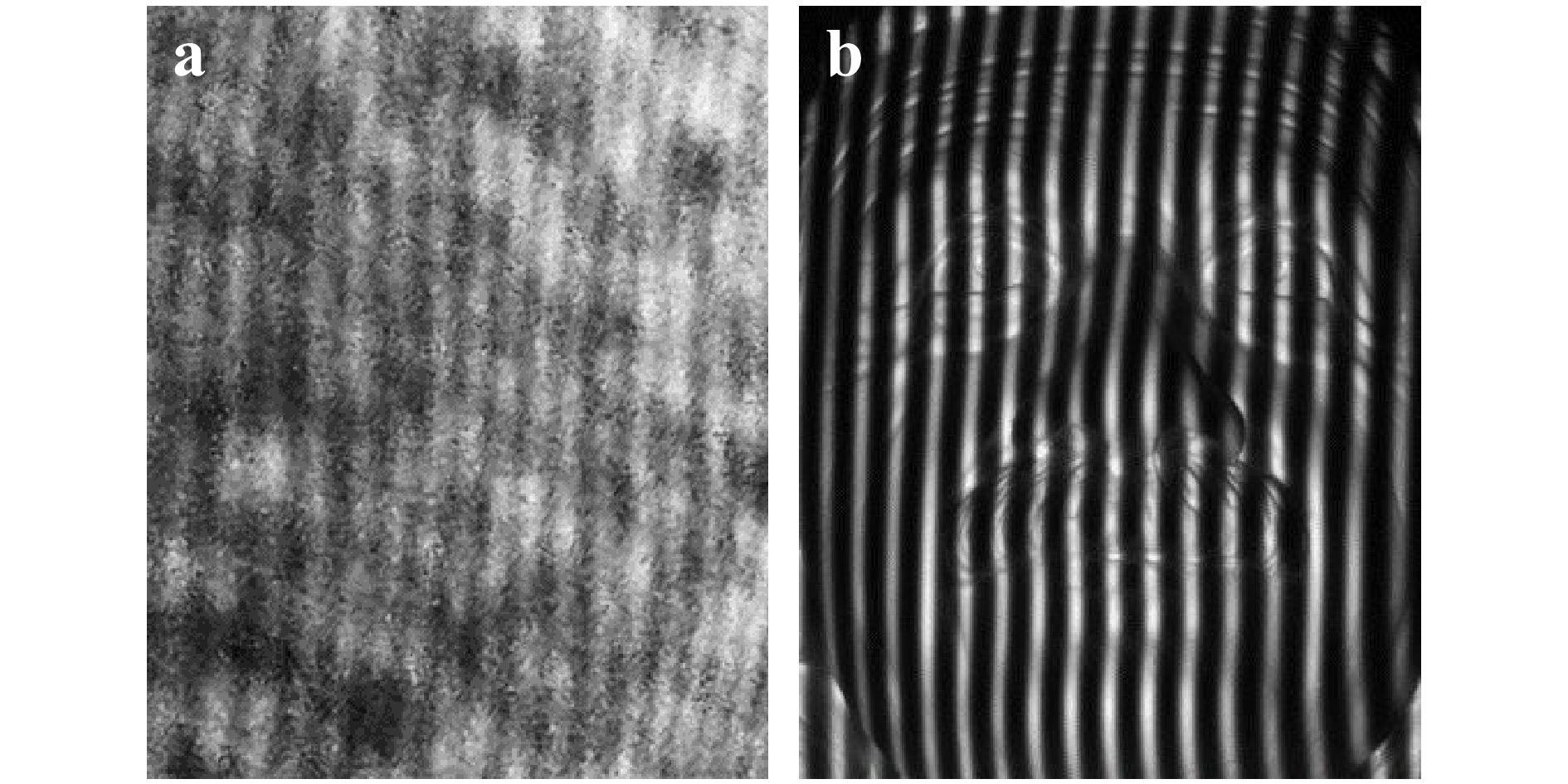

Fig. 2  Systems-theoretical similarity between holographic encoding and decoding in fringe projection triangulation: Both images can be decoded by single-sideband demodulation. a Close-up photograph of a transmission hologram recorded on photographic emulsion¹². b Fringe projection triangulation camera image for the measurement of the face of a plaster bust.

Even more, the decoding of a hologram is information-theoretically the same as the decoding process in single-shot fringe projection triangulation (“Fourier transform profilometry”^{14, 17}). Both are decoded by single sideband demodulation, implemented by optical separation of the zero-diffraction order from the $ +/- 1^{st} $ diffraction orders. Moreover, both methods share the same space-bandwidth limitations: only one-third of the available space-bandwidth can be used^{15, 18}. For the commonly static objects of holography and interferometry, it is standard to replace 2/3 of the expensive space bandwidth by temporal bandwidth via phase shifting¹⁹. However, temporal phase-shifting requires at least three subsequent exposures, which poses a serious problem for real-time metrology.

Single-shot measurements are possible, but not with a dense 3D point cloud. The simple reason is that one camera pixel cannot deliver the necessary information about the local illumination, the local reflectivity, and the distance $ z(x,y) $ of an object point.

Typically, single-shot sensors display point cloud densities much lower than 1/3 of the available pixels²⁰ as the available space bandwidth also needs to account for the solution of the so-called ‘indexing problem’. The “single-shot 3D movie camera”^{15, 20, 21} solves this problem with a trick that (from a systems-theoretical side) shows strong similarities to two-wavelength holography or -interferometry: Instead of a sequence of images taken at different wavelengths (or fringe-frequencies), two cameras simultaneously capture two images of the fringe-encoded surface from two different viewing angles. Interestingly, the decoding algorithms’ mathematical structure resembles those used in dual-wavelength interferometry^{20, 22, 23}.

So far, about the systems theory of encoding and decoding. Irrespective of the system theoretical similarities, the physics of the encoding is fundamentally different in both principles. In a hologram, the optical path-length and the reference wave encode the (interference) fringe phase, respectively the local distance $ z(x,y) $. In the triangulation system, the distance is encoded just by the perspective distortion of the fringe pattern projected onto the object surface, see Fig. 2.

Holograms of rough objects and the reconstructions display speckles which are a fundamental source of the uncertainty, not only for holographic metrology: Watching the seemingly noise-free triangulation image of Fig. 2b more carefully, it turns out that the fringe phase displays a small random error as well. This error is caused by the unavoidable partial spatial coherence of the illumination in combination with the observation aperture. There is always some residual spatial coherence, even with a large white incoherent light source, which results in an ultimate lower limit of the measuring uncertainty $ \delta z $ for the local distance z of an object point¹⁴. Fig. 3 illustrates the ‘ubiquitous spatial coherence’: Already partial spatial coherence disturbs measurements of rough surfaces, even if speckles are unnoticed by a distant observer with a small observation aperture. The ultimate uncertainty limit is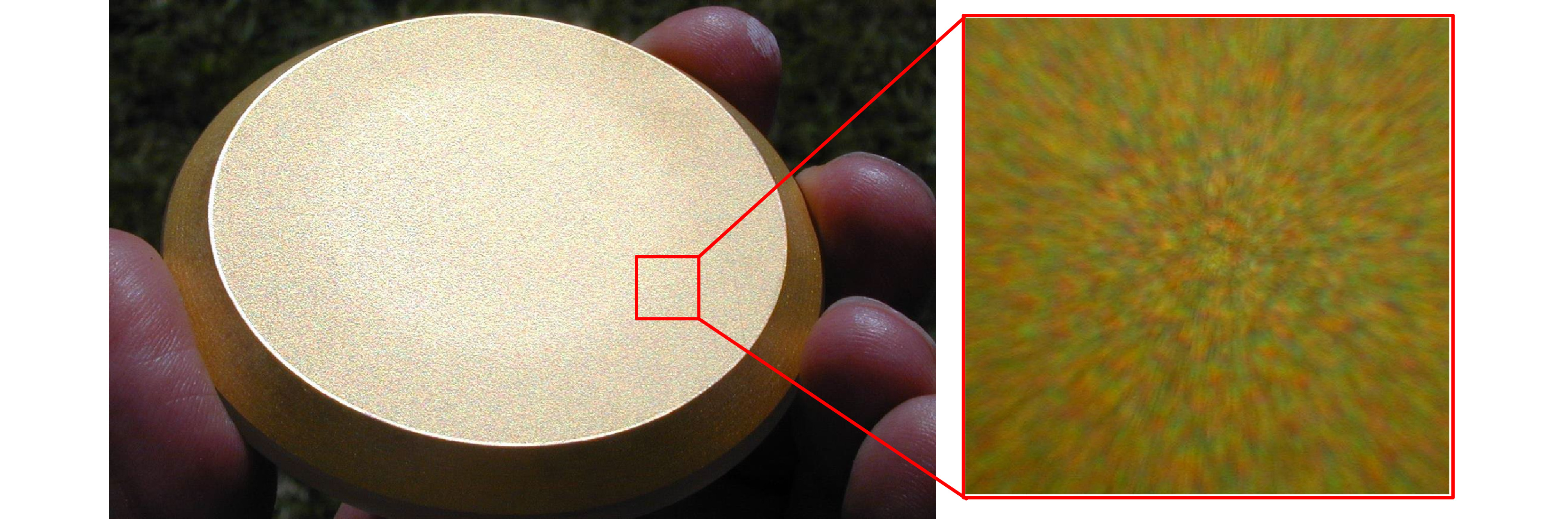

Fig. 3  Groundglass in sunlight: at close distance - with the observation aperture angle close to the illumination aperture angle - speckles can be seen even with a white extended light source.

where θ is the triangulation angle, $ \sin{u_{obs}} $ is the observation aperture and C is the speckle contrast ($ C=1 $ for laser illumination, so for most holograms). For focus-searching principles Eq. 1 degenerates to the Rayleigh depth of field (neglecting the C/2π factor), as $ u_{obs} $ acts as effective triangulation angle:

For spatially incoherent light sources, the contribution $ C_s $ of spatial coherence to the speckle contrast C can easily be estimated by the observation aperture and the illumination aperture²⁴ via:

For the other contributing factors polarization, temporal coherence and averaging via large pixels, see^{20, 24, 25}.

An illustrative daily life example: for laser triangulation (with $ C=1 $, $ \sin{u_{obs}} = 0.01 $, $ \sin{\theta} = 0.2 $) we achieve an uncertainty of about 40 µm. With spatially ‘incoherent’ fringe projection using a large incoherent illumination aperture (see Eq. 3), the same specifications may lead to a uncertainty about four times better.

These beneficial properties made fringe projection triangulation a well-established ‘gold standard method’ for many macroscopic applications. A well-designed sensor avoiding as much spatial coherence as possible may display a dynamical range of up to 10,000 depth steps. We emphasize that efficient metrology is enabled only by efficient source encoding. In optical metrology, illumination plays the role of the source encoder to encode the depth in an information-efficient way (with low redundancy)²⁶.

Coming back to holography: Can we decipher the surface topography from a hologram? At first glance, this should not be a problem, as we can “see” the 3D reconstruction (this marveling feature can hopefully be exploited for displays in the future). But what about exploitation for metrology? One could suspect that the object surface can be fully reconstructed within the limits of diffraction theory, where the size of the hologram can be seen as the limiting aperture. We approach the answer via an extreme counter-example: a hologram of a diffusely scattering white planar surface. It is impossible to find the surface by focusing through the hologram, as it is impossible to focus a camera onto a white wall in daylight. The deep reason is that the wave field in front of the holographic plate can be restored from the hologram, but (generally) we cannot localize the millions of surface points where the individual spherical waves have been scattered in the direction of the holographic plate. It will be discussed later that holography can access not just a wavefront but, after all, even the coherence function and the surface topography.

In turn, this means that some structure is necessary to acquire the object surface from a simple hologram, either via inherent features (salient points) or structured illumination as used in active triangulation. The structure is necessary for the holographic reconstruction and incoherent methods.

To summarize, we have to admit that although holography - as classical interferometry - encodes distance via the phase of the propagating waves, deciphering of the surface topography is not possible without additional information. Classical interferometry commonly looks at the image plane, so there is a priori information about the object’s location. Without such additional information, interferometric measurements can principally measure a wavefront but not the true surface of a remote object.

Even with ‘additional information’ there is a caveat. Here an illustrative example: from the image of a laser spot projected onto a rough object, the distance z can be found via focus search or shearing interferometry, despite speckle^{27, 28}. However, it was shown that both methods have to be attributed to class I, which possibly might surprise the reader. The explanation follows in “Holography versus slope measuring methods” section.

Triangulation of a rough surface with laser illumination suffers from a serious measuring uncertainty, determined essentially by the observation aperture: These properties can be looked up in Table 1. Triangulation measurements through a hologram and via indirect measurements by numeric backpropagation must also be attributed to class I. There is one exception: if the object displays fluorescence or is thermally excited, there is no speckle (and no hologram) because of perfect spatial incoherence^{29, 30}. Microscopy based on fluorescence microscopy can localize molecules with an uncertainty below nanometers.

Consequently, the ultimate uncertainty of holographic (rough surface) topography measurement via focus search (or related methods) is given by Eqs. 1 and 2, and depends strongly on the observation aperture (and not by the much lower photon noise of classical interferometry). Fortunately, by exploiting the large aperture that holography may easily provide, the uncertainty can be comparably high, despite speckle noise.

Phase randomization in speckle patterns forbids the topography measurement of rough surfaces with single-wavelength interferometry. A solution that is well established now is Coherence Scanning Interferometry (CSI). As mentioned in the introduction, the terms ‘rough-surface CSI’ or ‘coherence radar’^{10, 11, 31} are more substantiated.

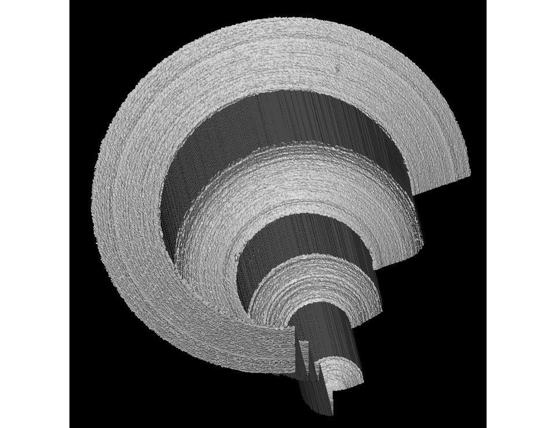
Fig. 4  Gauge for an injection nozzle (about 10 mm long), measured by rough-surface coherence scanning interferometry. Despite the low aperture that allows for measuring within deep holes, the measuring uncertainty is only a few micrometers.

A partial solution that holography can implement is two-wavelength holography, enabling the topography acquisition by contouring: A hologram of the surface is made by illuminating the object and the holographic plate with a wavelength $ \lambda_1 $. In a second step, the holographic plate and the object are illuminated with a wavelength $ \lambda_2 $, slightly different from $ \lambda_1 $. The object recorded at $ \lambda_1 $ is played back with $ \lambda_2 $ and superimposed with the wave from the object illuminated at $ \lambda_2 $. The interference pattern displays contour lines at a distance given by the “synthetic” wavelength³²⁻³⁶

which is the beat wavelength between $ \lambda_1 $ and $ \lambda_2 $ and hence can be picked orders of magnitudes larger. The light at the optical wavelengths $ \lambda_1 $ and $ \lambda_2 $ acts as a carrier for the synthetic wave. The optical wavelengths are scattered, meaning that the object serves as a “rough mirror” despite the large synthetic wavelength and the object can be seen from all directions. At the same time, the observed interference fringes at the synthetic wavelength do not display phase randomization. It is noteworthy that now, even a surface without features like edges or texture can be reconstructed. Bright contour lines are found where the two waves (with $ \lambda_1 $, $ \lambda_2 $) display the same phase. However, the temporal coherence function is periodic for two-wavelength holography, causing an ambiguous reconstruction. The ambiguity can be avoided by ‘multi-wavelength’ holography or white-light interferometry^{10, 35, 37}.

This remarkable advantage of two-wavelength interferometry and -holography has been utilized recently for the relatively new research field of “Non-Line-of-Sight” imaging, which is concerned with the task of looking around corners and imaging through scattering media. The method is based on the acquisition of a synthetic wavelength hologram which is taken by imaging a remote surface (such as a wall), that can “see” the hidden object and the sensor unit. This remote surface acts as a “virtual holographic plate”. The object is reconstructed by holographic backpropagation from the synthetic hologram at the synthetic wavelength^{35, 38, 39}. Following this procedure one can consider the wall as “rough mirror”.

After understanding the role of roughness qualitatively, again, the obligatory question: How to categorize two-wavelength holography in terms of noise? The resulting images with more or less ‘un-speckled’ fringes suggest an attribution to “classical interferometry”, characterized by photon noise as the cause of the uncertainty limit.

Combining the advantages of diffuse scattering with visible light illumination, without the drawbacks of speckle, sounds like magic, meaning that carefulness is advisable. And indeed, two-wavelength holography is not attributed to the same class as classical interferometry. Two-wavelength holography and -interferometry belong to class III, where the surface roughness ultimately limits the uncertainty: The reason is that the speckles produced by the two closely spaced wavelengths $ \lambda_1 $, $ \lambda_2 $ display a small phase decorrelation^{33, 35, 40} resulting in a random phase difference $ d\varphi_{1,2} $. This phase difference may correspond to a path difference of only $ \; \lambda/100 $ (for example). However, in the output signal, the measured path difference is “magnified” by $ \Lambda / \lambda $ resulting in a random distance error of $ \Lambda/100 $, instead of $ \lambda/100 $, in this example. This measuring uncertainty is much larger than the photon-noise limit of classical interferometry.

To estimate the random phase error and its physical cause, we assume that the two speckle patterns at $ \lambda_1 $ and $ \lambda_2 $ are sufficiently spatially correlated, as we select the synthetic wavelength to be much larger than the surface roughness^{35, 41}. At a certain image point (x', y'), waves are accumulated from a small object area given by the back-projected diffraction point spread function of the observing lens. This area will be approximately the size of a back-projected subjective speckle. The rough surface will have a ‘summit’ or peak within this area, and there will be the deepest valley point. The peak-valley distance $ R_t $ (over a certain length) is one of the common roughness parameters. $ R_t $ determines the maximum possible phase difference $ d\varphi_{1,2} $ between all waves accumulated within (x', y'). For the two wavelengths $ \lambda_1 $, $ \lambda_2 $, we easily find:

And with $ \delta z = \Lambda \cdot d\varphi_{1,2} / 2 \pi $ we get the measuring uncertainty at the position $ (x’, y’) $:

Eq. 6 tells us that the phase decorrelation between the two wavelengths limits the measuring uncertainty to a value given just by the surface roughness. Although an approximation, the physical cause of the measuring uncertainty is found. The same cause, even with a very similar quantitative result, was found in a rigorous analysis for rough-surface CSI^{42, 43}.

A few more clarifying words about rough-surface CSI ( ‘coherence radar’)^{10, 31}: The micro-topography of most “rough” surfaces such as a white wall, a ground glass, or a machined surface cannot laterally be resolved unless we use a high aperture microscope. Nevertheless, even with a small observation aperture, within deep boreholes and from a large distance, we can measure the roughness without laterally resolving the micro-topography. The roughness is given by the statistical measurement error $ \delta z $. As most daily life surfaces or technical objects have a roughness of only a few micrometers, the uncertainty of rough-surface CSI is much better than that of triangulation. As a further present, this uncertainty is independent of the observation aperture.

With the benefit of hindsight, the similarity of the physical cause of the dominating noise is not surprising, as both methods (scanning white-light interferometry and two-wavelength interferometry/holography), exploit an interplay of two (or more) wavelengths.

We summarize this section by assigning two-wavelength holography and two-wavelength interferometry to class III: These methods exploit just ‘time-of-flight’ or optical path length variations, so the ultimate limit of height uncertainty is given by the surface roughness and does not depend on the observation aperture^{8, 43}. Again, rough-surface CSI’s ultimate uncertainty is only determined by the object and not by the instrument, which is a remarkable physical and information-theoretical peculiarity.

A short appendix: It is well known that illumination by a wavelength significantly larger than the surface roughness helps measure rough surfaces. One could use far infrared light⁴⁴, but this creates a new problem: the surface now acts like a mirror (besides technical issues and the limited availability of infrared detectors). For 3D objects strongly deviating from a plane, the light will scarcely find its way back to the hologram plate/detector. It is important to note that the physical properties of such an experiment must be looked up under category II, “classical interferometry”, as the surface is smooth for the long wavelength. We see that changing the illumination may change the physical background dramatically.

The so far discussed methods intrinsically measure either the lateral position of a local feature (which is translated into distance via triangulation) or they measure the distance via an interferometric measurement of the phase (or time-of-flight) of a coherent (or partially coherent) signal. However, a class of physically completely different methods also exists - where the intrinsic signal is the local slope. ‘Intrinsic’ means that the slope is not evaluated by a-posteriori differentiation - the slope is already encoded in the optical signal before arriving at the photodetector. This is an invaluable feature, as the encoding is done optically before adding the detector noise. Hence, some of these methods enable sub-nanometer uncertainty for local surface height variation by very simple means. The reason is that intrinsic slope measurement corresponds to a perfect source encoding: the OTF represents the spatial derivative (or at least an approximation for shearing methods). Among the spatially differentiating methods, we find the so-called phase-measuring deflectometry (PMD)⁴⁵⁻⁴⁷, which is completely incoherent, and we find classical shearing interferometry⁴⁸.

Both methods measure specular surfaces or wavefronts. For rough surfaces, shearing holography comes into play, specifically because of its unlimited options for post-processing of the holographic data. We do not discuss the so-called “photometric stereo” here, as it commonly requires lambertian scatterers and is based on accurate intensity measurements. Hence, “photometric stereo” is sensitive against unavoidable spatial coherence, specifically because small light sources are used to generate shading.

In phase measuring deflectometry⁴⁵⁻⁴⁷, a large screen with an incoherently radiating sinusoidal fringe pattern is in remote distance from the specular object under test, see Fig. 5. The observer watches the screen that is mirrored by the object. If the object is not planar, the captured fringes in the camera image are distorted.

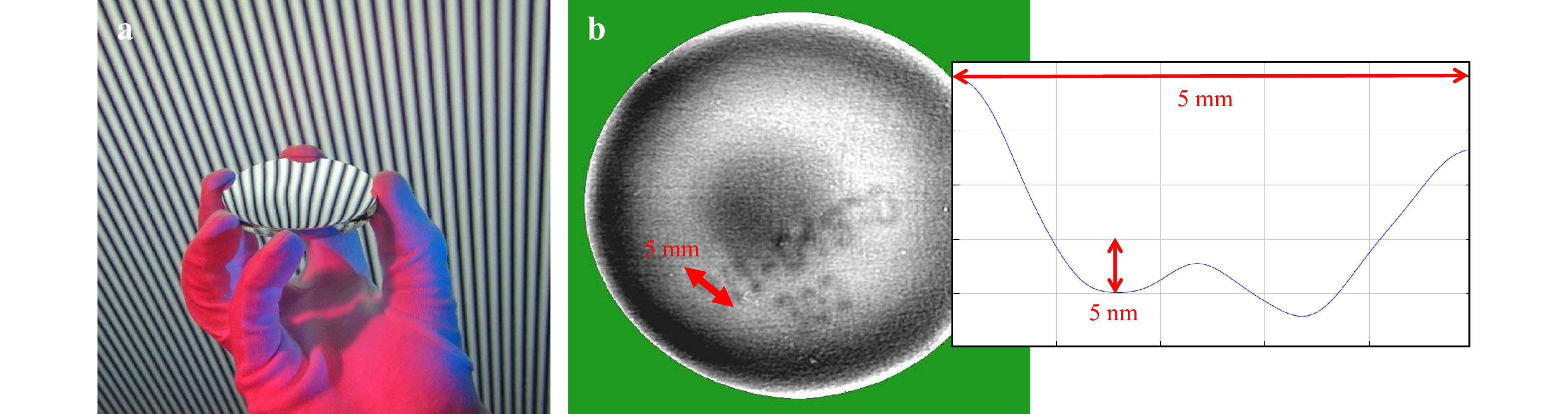
Fig. 5  Phase measuring deflectometry. a the basic principle, b “ghostwriting” depth map: A lens was marked with a whiteboard marker; later, the numbers were erased. The few nanometer damages of the lens surface can be detected and quantitatively evaluated.

Local surface deformations beyond the nanometer range can be measured from the distortion which is quantified by phase shifting. There is also a microscopic realization⁴⁹, where weak phase objects can be measured in transmission⁵⁰. There is very low spatial coherence with an incoherent (self-luminous) screen, and the method is essentially limited by photon noise. However, the ultimate limit of the height uncertainty depends on the lateral resolution as well, see Table 1. An interesting coupling of the angular uncertainty $ \delta \alpha $ and the lateral resolution $ \delta x $ leads to the useful uncertainty product given in Eq. 7. The camera must simultaneously focus on the object surface and the remote screen pattern (sinusoidal fringes). This depth-of-field problem requires a trade-off between angular uncertainty and lateral resolution⁵¹. More deeply, it is the Heisenberg uncertainty product that does not allow both a small $ \delta x $ and, at the same time, a small $ \delta \alpha $, for a single photon. However, the SNR and the height resolution are virtually unlimited with many photons. Together with the signal-to-noise ratio SNR, we get:

As an SNR = 500 can easily be achieved with standard video cameras, a depth uncertainty of $ \delta z = 1 \;{\rm{nm}} $ is possible with a piece of few-dollar equipment (λ is $ 500 \;{\rm{nm}} $). Similar considerations prevail to classical shearing interferometry, but this requires more costly equipment and does not deliver a true derivative. The ‘scaling’ of shearing interferometry is given by the wavelength of light, while some macroscopic fringe generator gives the scaling of incoherent deflectometry. Nevertheless, incoherent deflectometry can easily compete⁵¹, and both methods are limited by photon noise.

Eq. 7 offers numerous options: for a very low spatial resolution (e.g., for the measurement of a big flat mirror), the angular uncertainty can be in the micro-arcsec range⁵².

For the sake of completeness, we also mention the well-established Hartmann-Shack sensor as one more incoherent slope measuring sensor. It allows for direct measurement of wavefronts coming, e.g., from the pupil of a lens under test⁵³. A certain limitation is the wavefront sampling by an array of discrete lenslets.

Coherent differentiation is possible as well: Among the approximately “differentiating” methods, there is shearing interferometry and shearing holography^{54, 55}, including its numerous (more or less coherent) implementations such as the Nomarski differential interference contrast⁵⁶.

We move on to holographic shearing-interferometry, as it offers the possibility to measure the local slope of a rough surface. A wavefront is compared with a version of itself shifted (‘sheared’) by a distance s. A precious advantage of shearing methods (via a shearing plate) is the common-path geometry, being insensitive against environmental perturbations. Shearing holography is commonly realized via a shearing plate and captures several sheared interference patterns corresponding to different shears. The different shears correspond to different OTFs in the Fourier space. Hence, a hologram with a desired OTF can be synthesized by combining different interference patterns⁵⁷ and evaluated by numerical backpropagation.

To understand the physical limit of rough surface shearing holography, we refer again to the example of a projected laser spot^{27, 28}: A laser spot with diameter $ d_{spot} $ is projected onto the object. In the hologram plane, an objective speckle pattern with speckle diameter $ d_{speckle} \approx \lambda \cdot z / d_{spot} $ is generated and superimposed with a laterally shifted copy of itself. As far as the shear s is smaller than the speckle diameter, fringes can be seen, however, with some phase noise, due to the phase decorrelation within each speckle. Earlier investigations reveal that this phase noise leads to a measuring uncertainty $ \delta z \approx \lambda / \sin^2u_{obs} $, which is just the Rayleigh depth of focus (why are we not surprised?). Obviously, shearing interferometry at rough surfaces, as a tool to measure the local distance, displays (only) the same uncertainty limit as focus searching methods. Hence it belongs to class I. This is a result that a naïve observer possibly would not have expected: Shearing holography at rough surfaces is equivalent to triangulation to measure local distance.

The situation is even more difficult for an extended object and a large shear. Principally, each surface point generates a fringe pattern in the hologram, but the phase is random to other surface points, which makes the deciphering of the hologram difficult. Nonetheless, the object can be fully reconstructed from the holograms⁵⁷. The basic idea here is to determine the complex-valued coherence function from the recorded interference patterns, starting from the mixed interference term $ E^*(x,y) E(x+s,y) $ of the complex signal E. From there, one can reconstruct finite differences of the wavefield corresponding to positions separated by the shear or by combining several shears, the non-differentiated wavefront.

A real finite difference can be achieved by using “Γ-profilometry”, which exploits the temporal coherence function⁵⁸. The method is strongly related to rough-surface CSI, as described in “Holography versus rough-surface interferometry” section. A significant difference to scanning white-light interferometry is that the outcome here is not the surface profile $ z(x,y) $ but the difference $ \Delta z = z(x,y)-z(x+s,y) $. This property can be an advantage, as for most objects, the depth scanning time will be significantly lower, as the scanning range is limited by the maximum of $ \Delta z $ instead of the full object depth range. Γ-profilometry is an illustrative example of redundancy reduction via source encoding. It follows from these considerations that the roughness of the surface gives the ultimate source of noise for Γ-profilometry with broadband illumination: The method has to be assigned to class III, again with the useful feature that the measurement uncertainty does not depend on the observation aperture. Apparently, it is a fruitful idea to “copy” and possibly improve established methods like rough surface CSI by proper holographic storage and the big toolbox of computational evaluation.

Eventually, the so called ‘shearography’⁵⁹ has to be mentioned: Speckle shearography takes advantage of the common path geometry of shearing interferometry. The robustness against environmental perturbation is exploited to measure very small (temporal) changes of the surface “slope”, the sensitivity depending on the shear. The method is, of course, sensitive against speckle decorrelation. For deformations close to a wavelength, phase decorrelation probably dominates. So only under the assumption of very small surface changes might the uncertainty be limited by photon noise.

We have set aside this consideration until now, hoping that the preceding sections simplify the understanding: As far as specular surfaces are involved, holography belongs to class II, classical interferometry, due to the fact that here the uncertainty is limited by photon noise.

For holographic interferometry at rough objects, the object is compared with a slightly deformed version of itself. As discussed for speckle shearography, the phase in two highly correlated speckles is compared. As far as there is very low decorrelation, the uncertainty is limited by photon noise, as for classical interferometry. However, this is not a binary decision, as phase decorrelation and fringe delocalization occur with increasing deformation.

Holography is a tool to store complex wavefronts and to process the data either optically or by computation. There are numerous implementations - amongst others - to acquire data about the topography of an object's surface, which is the focus of this paper. The comparison of holographic methods with non-holographic methods offers some interesting insights. The first insight is that holographic methods can be assigned to one of four classes defined via the physical cause of the dominant noise and the dependence of the observation aperture. As not every method is investigated, the authors admit that further discussion might get new insights.

Methods based on triangulation are seriously disturbed by speckle, with the consequence that holography is not the first choice to measure surface topography via triangulation, e.g., by focus search or related methods. 3D metrology, based on triangulation, is the turf of incoherent methods, at least for macroscopic objects. Many microscopical objects are weak phase objects, and there is no clear distinction between defocusing noise and speckle. Furthermore, the observation aperture can be extremely high - so with the help of Eq. 2, holographic methods often deliver acceptable results despite some coherent noise.

We think that holographic interferometry aiming to measure sub-λ deformation, is the natural realm of holography, where most incoherent methods fail.

Furthermore, two- or multi-wavelength holography might potentially become a competitor of the corresponding non-holographic methods that we find in the class “rough-surface interferometry”. The potential of holography is strongly related to the vast realm of computational options. ‘Seeing around the corner’ is only one striking example, where several holographic ideas are combined.

Among the methods that intrinsically measure the slope, (incoherent) phase measuring deflectometry has become an invaluable tool to measure virtually any kind of specular surface, even competing with interferometry⁵⁴. Deflectometry displays an extreme sensitivity for local surface defects, with at the same time low hardware requirements. Can holography compete? Maybe for rough surfaces: Among the (approximately) differentiating holographic methods, multi-wavelength shearing-holography seems to be a proper method to measure the slope of rough surfaces. Again, the virtually unlimited options for computational post-processing are an advantage over “purely” optical methods. The uncertainty limit is determined just by the surface roughness, the same limit as rough-surface interferometry.

We conclude by stating that holography offers the presentation of breathtaking 3D images. The underlying storage of a complex wavefield, together with virtually unlimited options for processing by computation, is breathtaking as well. As there will be many not yet invented algorithms, future researchers might profit from knowing and exploiting the fundamental limits to exploit holography better.

The authors gratefully acknowledge numerous intriguing discussions with Claas Falldorf (BIAS Bremen) and Christian Faber (Hochschule Landshut), and as well their critical reading of the manuscript.