Towards multi-dimensional atomic-level measurement: integrated heterodyne grating interferometer with zero dead-zone

With the rapid advancement of the global semiconductor and electronic information industries, industrial production is increasingly trending toward greater intelligence, miniaturization, high speeds¹, and enhanced integration². Components in precision-driven sectors, such as lithography systems, atomic-scale manufacturing³, and quantum technologies⁴, have reached atomic-level precision, placing stringent requirements on industrial manufacturing processes⁵. As a fundamental enabler of high-end industrial manufacturing, precision measurement technology must now deliver extremely high accuracy, achieving sub-nanometer or even picometer precision in certain fields^{6, 7}. Furthermore, advanced measurement technologies are required to address emerging demands for environmental robustness, multi-degree-of-freedom (multi-DOF) functionality, and advanced error elimination⁸.

Current precision measurement technologies include capacitive sensors⁹, time grating sensors¹⁰, laser interferometers¹¹, and grating interferometers¹²⁻¹⁴. Although capacitive sensors are capable of achieving sub-nanometer accuracy, their measurement range is limited to the millimeter scale¹⁵, which constrains their applicability in large-scale systems. Time grating sensors offer linear displacement measurements with an accuracy of approximately hundreds of nanometers¹⁶. Laser interferometers can attain sub-nanometer precision over meter distances but are highly sensitive to reflector quality and environmental conditions, which can introduce errors in multi-DOF configurations^{17, 18}. In contrast, grating interferometers exhibit greater robustness against environmental disturbances and are capable of generating multi-level interference fringes, and thus excel in high-precision and multi-DOF measurements across extended ranges¹⁹.

Based on the type of laser source, grating interferometers can be classified into homodyne²⁰⁻²² and heterodyne^{23, 24} systems. Homodyne systems utilize a single-frequency laser source that generates a direct-current (DC) displacement signal²⁰. In contrast, heterodyne systems employ dual-frequency laser sources that produce alternating-current (AC) displacement signals. Compared to homodyne systems, heterodyne configurations generally offer higher accuracy and enhanced resistance to interference²³, making them particularly well-suited for nanometer or sub-nanometer measurement scenarios. However, due to the use of numerous optical components, heterodyne systems are prone to nonlinear errors that can compromise measurement accuracy²⁴⁻²⁶. Two primary sources of these errors are frequency and polarization aliasing^{25, 26}, as well as multi-level ghost reflections^{27, 28}, with the former having a greater impact.

To mitigate nonlinear errors caused by frequency and polarization aliasing, researchers have focused on two primary approaches: spatially separated structures and algorithmic compensation. The former addresses the error at its source and is discussed below. The spatially separated structure separates the dual-frequency laser source at the incident section, ultimately enabling beat frequency interference. This approach avoids the frequency and polarization aliasing typical of traditional common-path systems, thereby significantly reducing periodic nonlinear errors. Wu et al.²⁹ pioneered a spatially separated heterodyne laser interferometer, reducing periodic nonlinear errors to 20 pm. Building on this, Guan et al.³⁰ proposed a differential interference heterodyne encoder that employs spatially separated input beams to eliminate polarization mixing. More recently, Xing et al.³¹ proposed a spatially separated heterodyne grating interferometer in which two modulated beams are transmitted through separate optical fibers, further reducing periodic nonlinear errors.

Nevertheless, spatially separated paths can introduce a dead-zone error due to differences in propagation distance, which exacerbates measurement errors resulting from laser source frequency instability and environmental noise. In response, some researchers have investigated designs aimed at minimizing dead-zone errors at their source. Fu et al.³² proposed a symmetric heterodyne interferometer that balances the probe and reference optical paths, effectively eliminating dead-zone errors and periodic nonlinear errors. Recently, Wang and Gao³³ developed a quasi-common-path heterodyne grating interferometry system incorporating oblique incidence and wavelength stabilization, thereby reducing periodic nonlinear errors to 0.3 nm while maintaining high resolution and improved interference immunity. For simultaneous in-plane and out-of-plane measurements, Hsieh et al.³⁴ designed a three-DOF grating interferometer utilizing a transmission-type two-dimensional grating, achieving nanometer-level resolution across millimeter-scale ranges. Lin et al.³⁵ introduced a wide-range three-axis grating encoder that provides nanometer resolution and an extended Z-axis range. However, most existing methods are unable to simultaneously measure in-plane and out-of-plane displacements with low nonlinear errors, limiting their applicability in large-scale, atomic-level measurement scenarios.

In response to these demands, this study presents a novel heterodyne grating interferometer geared toward multi dimensional, atomic-level precision measurements. The main contributions of this work are outlined as follows:

1. Development of a 3-DOF Heterodyne Grating Interferometer: A heterodyne grating interferometer is proposed, utilizing a dual-frequency laser source to enable the simultaneous measurement of three DOFs. An integrated prototype, with dimensions of 90 × 90 × 40 mm³, was fabricated to demonstrate both its feasibility and compactness.

2. Zero Dead-Zone Optical Path Design: A zero dead-zone optical path configuration was carefully designed to eliminate nonlinear errors at their origin, thereby enhancing measurement reliability. This design significantly reduces the influence of laser source frequency fluctuations and variations in air refractive index.

3. Global Crosstalk Error Analysis and Robust Correction: A comprehensive crosstalk error analysis was performed across different axes, and a robust correction algorithm was developed by integrating wavelet transforms with Butterworth filtering. The proposed algorithm reduces crosstalk errors to below 5%, thereby significantly enhancing measurement accuracy.

4. Comprehensive Performance Testing of the Integrated Prototype: The integrated prototype was subjected to rigorous evaluations, including assessments of resolution, linearity, repeatability, stability, and measurement range. Comparative analysis with representative industrial and academic measurement systems demonstrated the superior performance and reliability of the prototype.

The framework of the proposed 3-DOF zero dead-zone heterodyne grating interferometer is shown in Fig. 1, and its components are described in detail below.

Fig. 1  Framework of a grating interferometer system for 3-DOF measurement. a Reading head. b Calculation module. (c) Dual-frequency laser source. PPLN: Periodically Poled Lithium Niobate; HWP: Half-Wave Plate; QWP: Quarter Wave Plate; COL: Fiber Coupler; AOM: Acousto-Optic Modulator; P: Polarizer; PBS: Polarizing Beam Splitter; PD: Photo Detector; AD: Analog-to-digital conversion; CLK: Clock signal; FPGA: Field Programmable Gate Array; 0, $ X_{+1} $, $ X_{-1} $, $ Y_{+1} $, and $ Y_{-1} $ represent interference signals in five directions, respectively.

(1) Dual-frequency laser source: As shown in Fig. 1c, the system employs a 1560 nm rubidium atomic seed laser. The laser output is amplified by a power amplifier and then passed through periodically poled lithium niobate (PPLN), which converts the wavelength to 780 nm. The converted laser is subsequently coupled into an Acousto-Optic Modulator (AOM), generating two laser beams with frequencies $ f_1 $ and $ f_2 $.

(2) Reading head: As shown in Fig. 1a, the two lasers $ f_1 $ and $ f_2 $, possessing a frequency difference of $ f_0 = f_1-f_2 $, pass through a Half-Wave Plate (HWP) and a Polarizer (P) before entering a Polarizing Beam Splitter (PBS). Each laser beam is incident on its respective grating (with a 1000 nm period and 2D reflective grating): $f_1$ interacts with the measurement grating, while $f_2$ interacts with the reference grating. These gratings diffract the incident laser into five distinct beams: the 0-th order diffraction beam, first-order diffraction beam (X-axis positive), first-order diffraction beam (X-axis negative), first-order diffraction beam (Y-axis positive), and first-order diffraction beam (Y-axis negative). Finally, the ten diffracted beams interfere on the photodetector (PD) after passing through additional optical components such as the prism, HWP, QWP, and P. This interference produces five beat frequency (also referred to as heterodyne) interference signals, as illustrated in Fig. 1a, namely, 0, $X_{+1}$, $X_{-1}$, $Y_{+1}$, and $Y_{-1}$), with a frequency of $f_1-f_2$. For clarity, we added the laser propagation path in the lower left corner of Fig. 1a.

Next, we analyzed the polarization states of the beams. First, for laser $ f_1 $, after passing through HWP1 and P1, it becomes a p-polarized beam. It then passes through PBS1 and, after passing through QWP1, is converted into circularly polarized beam. The beam then undergoes reflection and diffraction at the diffraction grating. The five output beams are reflected back through QWP1, becoming s-polarized beam. Consequently, the beam is reflected at PBS1, passes through HWP3, where it is converted into p-polarized beam, and then transmitted through PBS2. After passing through P3, it is split into equal parts of p- and s-polarized beam. Next, we analyzed $ f_2 $. This beam follows a similar path, passing through HWP2, P2, PBS2, QWP2, the diffraction grating, QWP2 again, PBS2, and P3. After passing through P3, the beam is split into equal parts of p- and s-polarized beam, which then interfere with the corresponding components of laser $ f_1 $ to form interference signals (0, $X_{+1}$, $X_{-1}$, $Y_{+1}$, and $Y_{-1}$).

(3) Calculation module: As illustrated in Fig. 1b, the five interference signals are input into a field programmable gate array (FPGA) after undergoing signal conditioning and analog-to-digital (AD) conversion. The FPGA is responsible for calculating the 3-DOF displacement results. The principles of displacement calculation within the FPGA involve two main steps: OPL and SPD. The orthogonal phase-locking (OPL) method is used to determine the phase variation of the five interference signals over time. This process includes several steps: signal decomposition, mixing and filtering, phase extraction, and phase locking. Once the phase changes are obtained through the OPL method, the 3-DOF displacement xyz of the measurement grating is calculated using the symmetry phase differential (SPD) method.

The detailed principle of this calculation is presented in the “Measurement Principle, Eq. 3” below. Finally, the calculated displacement values xyz are transmitted to the host computer via Ethernet for real-time display.

This section explains how to determine the 3-DOF displacement of the measurement grating using the five interference intensity signals $ I_{0} $, $ I_{X_{+1}} $, $ I_{X_{-1}} $, $ I_{Y_{+1}} $, and $ I_{Y_{-1}} $ on the PD. Their expressions are as follows:

where $ i $ indicates $ 0 $, $ X_{+1} $, $ X_{-1} $, $ Y_{+1} $, and $ Y_{-1} $, $ I_{i} $ represents the intensity of the $ i $-th order interference signal, $ U_i $ denotes the amplitude of the $ i $-th signal, and the variable $ f_0 $ denotes the frequency difference between the two laser beams. $ {\Phi}_{i} $ and $ D_{i} $ represent the phase difference induced by the displacement of the grating and the phase difference caused by the dead-zone, respectively. Based on the Doppler effect and the grating equation, the expression for $ {\Phi}_{i} $ is as follows:

where $ \lambda $ represents the wavelength of the laser; $ x $, $ y $, and $ {\textit z} $ represent the displacements of the grating along the XYZ axes, respectively; $ \theta $ is the 1-st diffraction angle of the grating; $ n $ represents the refractive index of air; and $ g $ represents the grating period.

where the 1-st angle of the grating $ \theta $ is represented by $ \lambda $ and $ g $ through the grating equation. In this context, the 3-DOF displacement of the grating can be calculated from the phase change $ {\Phi}_{i} $ detected by PD.

As seen from Eq. 1, the phase change detected at the PD consists of two components: the grating displacement-induced phase variation $ \Phi $ and an additional phase term $ D $ introduced by the dead-zone error.

(1) Mathematical and Physical Concept of Dead-Zone

The dead-zone phenomenon arises from the optical path difference (OPD) between two interfering beams, causing inconsistent responses to environmental perturbations such as fluctuations in the air refractive index and laser frequency instability. This OPD-induced discrepancy results in an additional phase error, which ultimately reduces the accuracy of displacement measurements.

Fig. 2 schematically illustrates the concept of the dead zone, with certain optical components omitted for clarity. The optical configuration involves two laser beams with frequencies $ f_1 $ and $ f_2 $, propagating along distinct paths: (1) Measurement optical path: $ f_1 $ interacts with the measurement grating, which carries displacement information, and then combines with $ f_2 $ to produce a heterodyne interference signal, with its phase denoted as $ \Phi_m $). (2) Reference optical path: $ f_1 $ and $ f_2 $ are combined directly through optical components to generate a reference signal, with its phase denoted as $ \Phi_r $.

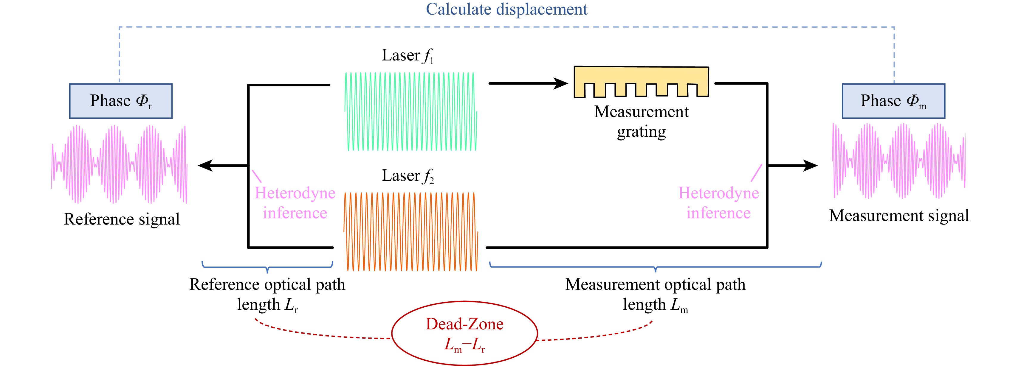
Fig. 2  Schematic diagram of the dead-zone in a grating interferometer. For clarity, the optical components in the measurement optical path and the reference optical paths are omitted, and only their physical path lengths are considered.

The dead-zone error is quantified by the path length difference $ \Delta L = L_m - L_r $, which makes the two optical paths differentially susceptible to environmental fluctuations. This differential sensitivity introduces an additional phase error $ D(t) $, which affects the measurement precision. The analytical expression for $ D(t) $ can be derived as follows.

For laser frequencies $ f_1(t) $ and $ f_2(t) $ propagating through a medium with a time-varying refractive index $ n(t) $, the phase delay experienced by each beam is given by:

where $ L $ indicates the geometric path length and $ c $ represents the speed of laser in vacuum. The phase differences for the reference and measurement paths can then be expressed as:

The resultant phase error $ D(t) $ is then expressed as:

where $ L_r - L_m $ denotes the length of the dead-zone, $ f_1(t) $, $ f_2(t) $, and $ n(t) $ are time-dependent quantities with stochastic characteristics that cannot be precisely measured, thereby serving as intrinsic sources of error. Eq. 7 reveals that $ D(t) $ depends on the instantaneous values of both the frequency difference and the refractive index, with its temporal evolution governed by their respective time indices. It is important to note that this expression is valid under the assumption that the dead-zone length, $ L_r - L_m $, remains fixed and unaffected by external disturbances. This assumption ensures the applicability of the expression under the condition of a constant dead-zone length, as detailed in Eq. 4 to Eq. 7.

(2) Methods to Eliminate Dead-Zone Error

To eliminate errors arising from laser frequency drift and refractive index fluctuations, minimizing $ L_r - L_m $ to zero is the optimal solution. The following section presents an optical design methodology that enables simultaneous 3-DOF displacement measurement while effectively eliminating the dead-zone error through precision path matching.

To address this challenge, the optical path in this study is meticulously designed to eliminate the dead-zone error. Fig. 3 illustrates the propagation path of laser within the XOZ plane, allowing for the calculation of the optical dead-zone for $ PD_{X_{+1}} $, $ PD_0 $, and $ PD_{X_{-1}} $ (from bottom to top on the right side of Fig. 3). The dead-zone formulas for the signals detected at $ PD_{X_{+1}} $, $ PD_0 $, and $ PD_{X_{-1}} $ are given as follows:

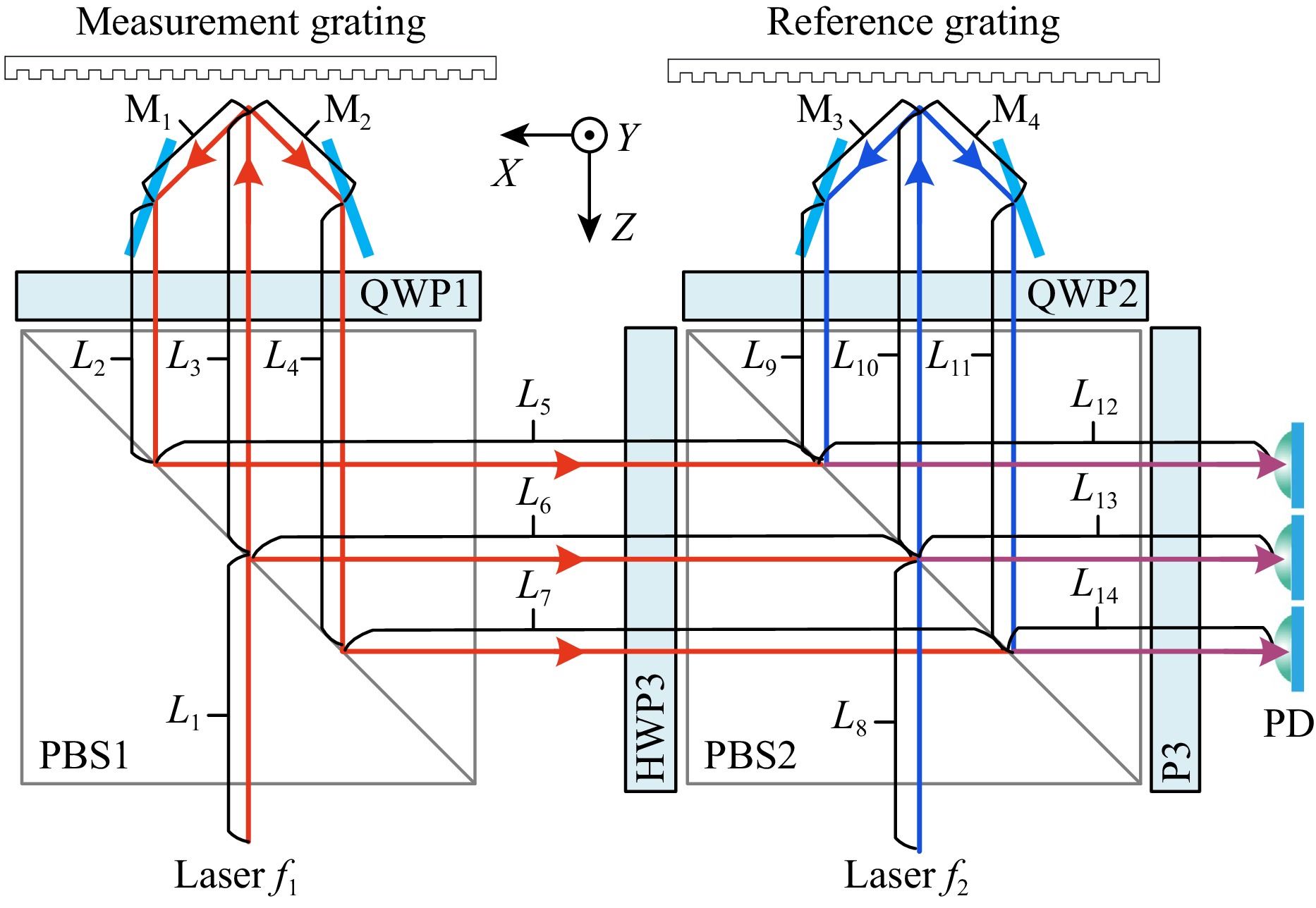
Fig. 3  Laser propagation path in the XOZ plane. L and M represent the optical path length of the respective beams.

where the optical paths are arranged in a spatially symmetric configuration, as illustrated in Fig. 3, leading to the following relation:

Further, by combining Eq. 3 and Eq. 7, the $ xy{\textit z} $ measurement error caused by the dead zone can be expressed as follows:

where the variables $x_{error}$, $y_{error}$, and ${\textit z}_{error}$ represent the measurement errors induced by the dead-zone. By simultaneously solving Eq. 9 and Eq. 10, we can derive the following:

which is equivalent to achieving a zero dead-zone condition in the system. In summary, the proposed optical path configuration fundamentally eliminates the dead-zone error at its source, thereby providing a solid foundation for multi-DOF displacement measurements with sub-nanometer-level or even atomic-level precision.

To verify the effectiveness and practical ability of the proposed system, an experimental setup was constructed, as shown in Fig. 4. A detailed description of the system components and configuration is provided below.

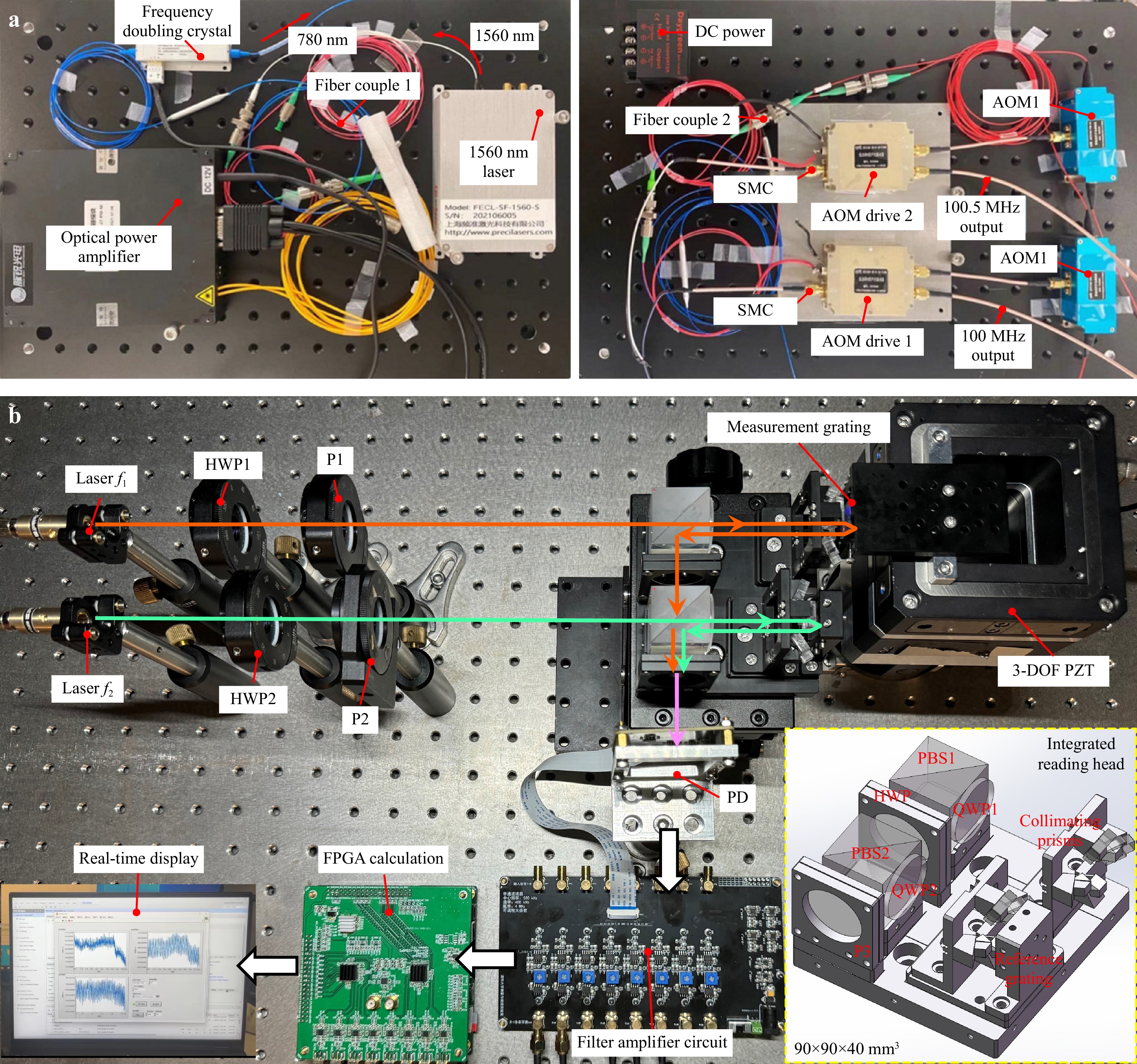
Fig. 4  Prototype of the grating interferometer system for 3D measurement. (a) Heterodyne dual-frequency laser source. (b) Measurement system, comprising the laser power control module (HWP and P), Integrated reading head, 2D measurement grating, 3-DOF Piezoelectric Stage (PZT), and a real-time processing and display module (PD, filter amplifier circuit, FPGA calculation and real-time display module).

Laser Source: As shown in Fig. 4a, the laser source module comprises both the generation and frequency modulation of the laser. First, the rubidium atomic seed laser source generates a 1560 nm laser, which is then passed through a power amplifier and a PPLN crystal to generate a 780 nm laser. Next, AOM1/AOM2, along with their driving circuits operating at 100.5 MHz and 100 MHz, respectively, modulate the laser frequency to produce laser $ f_1 $ (frequency: 100.5 MHz) and $ f_2 $ (frequency: 100 MHz), resulting in a frequency difference of 500 KHz. Finally, fiber coupling is employed to guide the laser beam from the laser source to the measurement system.

To assess the performance of the laser source, we used a beam profiler to analyze the laser, as shown in Fig. 6. As shown in Fig. 6a, the laser beam exhibits an elliptical intensity distribution, with widths of 4100.5 µm (X-4$ \sigma $) and 3322.9 µm (Y-4$ \sigma $). Fig. 6b shows that the maximum intensity peak is located at (0, 0) with a value of 100%, the 50% intensity points are at (0, 715.27 µm) and (1469.2 µm, 0). The energy center stability of the beam is controlled at (3.36 µm, 1.80 µm). In summary, the beam cross-section of the laser source exhibits an elliptical Gaussian distribution and demonstrates high stability, making it suitable for high-precision measurement.

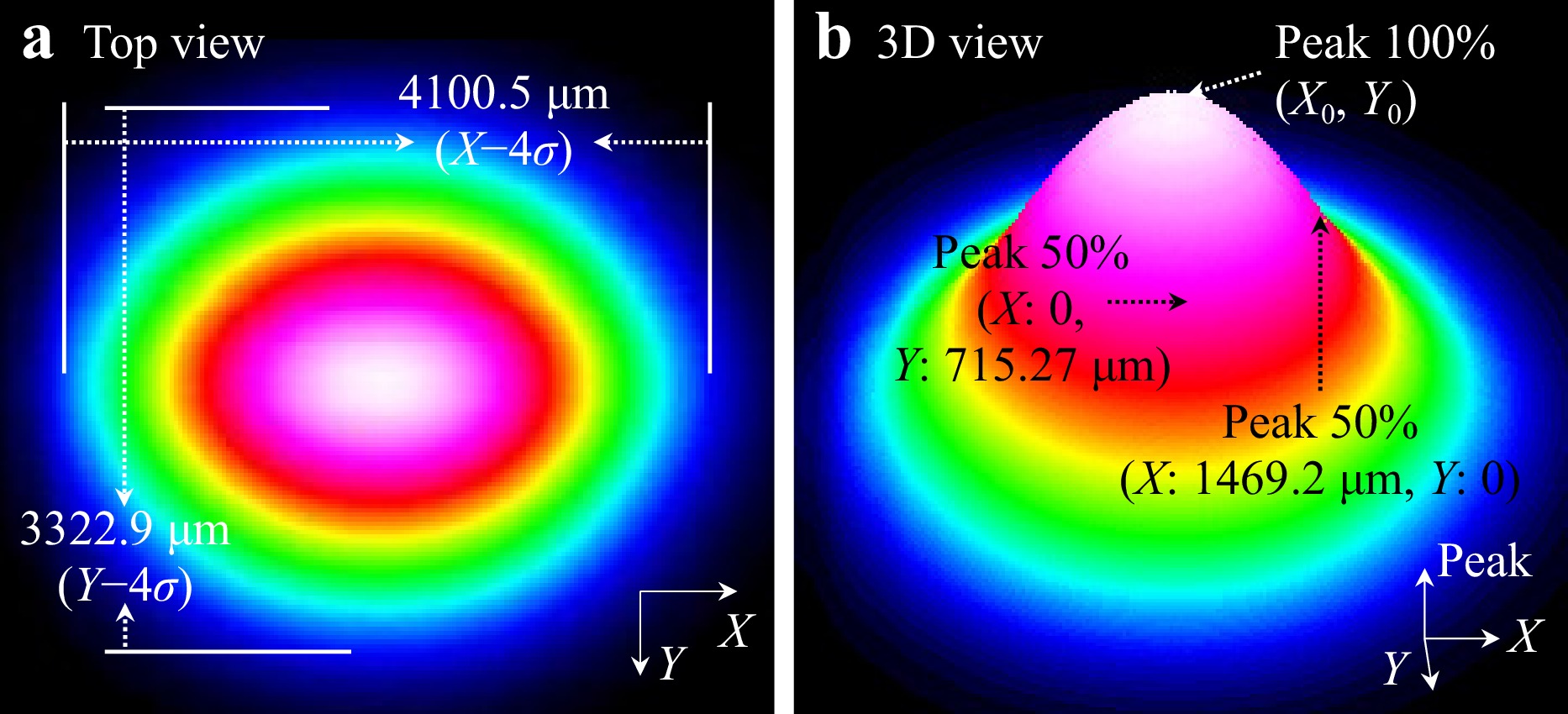
Fig. 6  Beam profiler test results of laser source. a Top view of the beam. b 3D view of the beam.

Measurement System: As illustrated in Fig. 4b, the laser beams, $ f_1 $ and $ f_2 $, pass through a series of optical components, including HWP and P to adjust their polarization states and energy. Subsequently, the beams interact with the measurement grating, and the reflected or diffracted beams propagate through an integrated reading head, where they are detected by a PD. The measurement grating is mounted on a 3-DOF PZT (a PI stage (P-733.2CD) for X/Z-axis motion and a PI stage (P-733.Z) for Y-axis motion), enabling precise displacement control. The integrated reading head integrates key components such as PBS, QWP, and a collimating prism, and is assembled into a compact 90 × 90 × 40 mm³ module. The signals detected by the PD are first amplified and filtered by a dedicated amplifier circuit, then transmitted to the FPGA for real-time processing. The measurement results are presented on a real-time display monitor, clearly indicating the 3-DOF displacement of the grating. Several sets of experiments will be conducted to evaluate the performance of the system, as described in the following sections.

(1) Resolution: Resolution refers to the system’s ability to detect the smallest measurable displacement. Fig. 5a, b show the extreme resolution tests for both in-plane (X/Y-axis) and out-of-plane (Z-axis) displacements, respectively. The tests were conducted under quasi-static conditions, with the stage moving at 1 μm/s in stepwise increments. The top graph illustrates the in-plane measurement with a step size of 0.25 nm, while the bottom graph depicts the out-of-plane measurement with a step size of 0.3 nm. These results demonstrate that the measurement system can resolve displacements in the range of 0.25 to 0.3 nm.

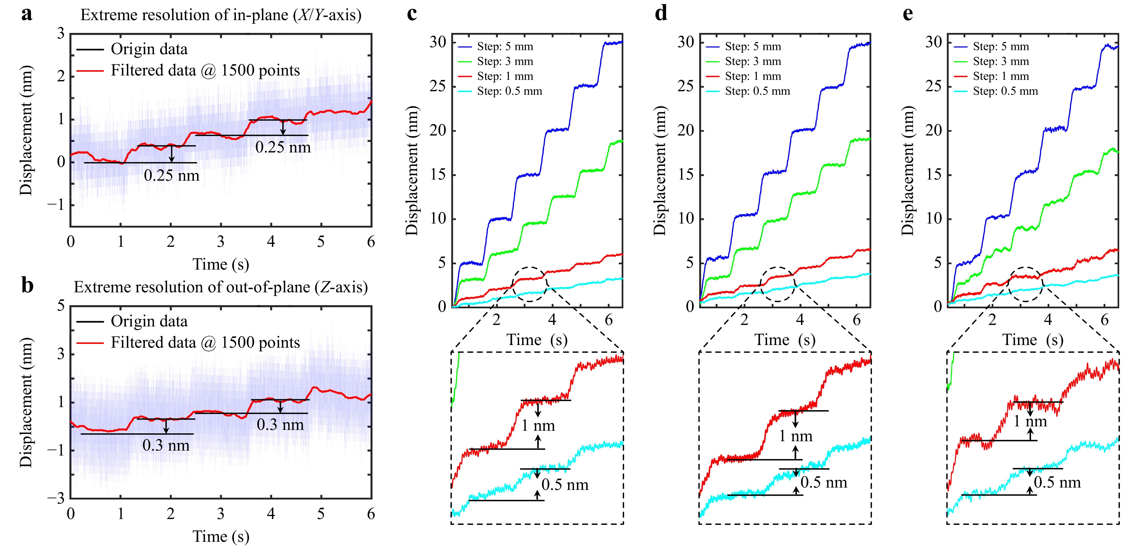
Fig. 5  Resolution test. a Extreme resolution test for in-plane displacement (XY-axis). b Extreme resolution test for out-of-plane displacement (Z-axis). c Multi-level resolution test along the X-axis. d Multi-level resolution test along the Y-axis. e Multi-level resolution test along the Z-axis.

Besides, Fig. 5c-e presents multi-level resolution tests for the XYZ axes, incorporating step sizes of 0.5, 1, 3, and 5 nm. In summary, the above experiments demonstrate that the system can resolve displacements at a near-atomic level (0.25 to 0.3 nm) and exhibits high universality across a wide range of displacement step sizes.

(2) Linearity: Linearity represents the error level of the measurement system across a defined measurement range. In Fig. 7, linearity tests were carried out for each axis. The calculation method involves subtracting the internal output value of the 3-DOF PZT (which was professionally calibrated to sub-nanometer precision and can be regarded as the “ground truth”) from the corresponding output value of the measurement system. Fig. 7a represents the directions of different axes, and the measurement range of each axis is 100 µm (this is the maximum stroke of 3-DOF PZT). For the linearity of the X-axis, as shown in Fig. 7b, the maximum and minimum errors observed are 4.8 nm and -6.9 nm, respectively. The error level during the stationary phase is 2 nm. For the linearity of the Y-axis, as shown in Fig. 7c, the maximum and minimum errors observed are 8.1 nm and -5.5 nm, respectively. The error level during the stationary phase is also 2 nm. For the linearity of Z-axis, as illustrated in Fig. 7d, the maximum and minimum errors are 16.1 nm and -16.2 nm, respectively. The error level during the stationary phase is 5 nm. Thus, the linearity of the XYZ-axis is calculated to be 6.9e-5@100 µm, 8.1e-5@100 µm, and 16.2e-5@100 µm, respectively. In the stationary phase, the linearity of the XYZ-axis can be improved to 2e-5@100 µm, 2e-5@100 µm, and 5e-5@100 µm, respectively. These results confirm the system’s high measurement precision, with the observed maximum deviations reflecting its non-linear characteristics.

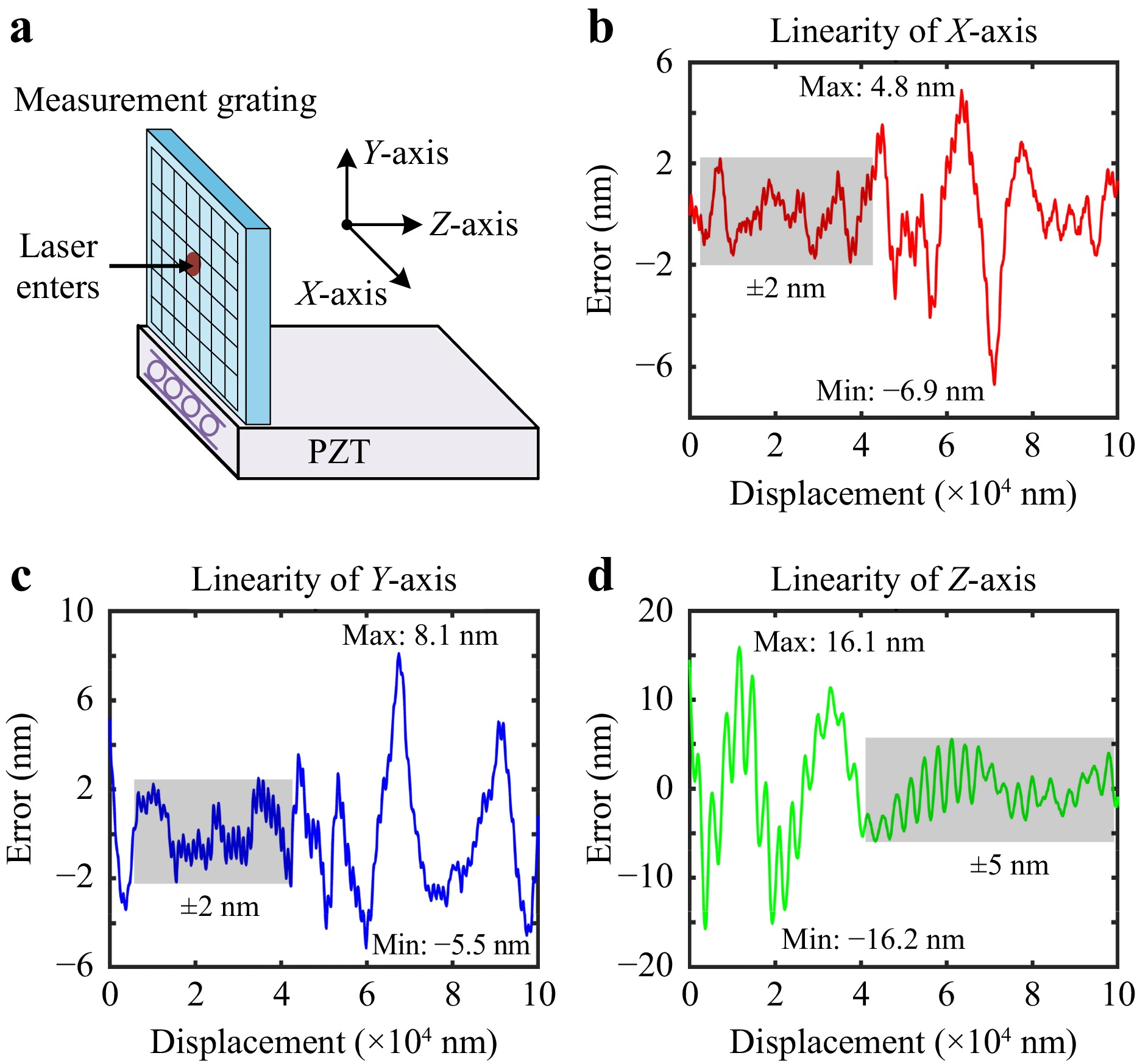
Fig. 7  Linearity test. a Schematic diagram showing the directions of different axes. b Linearity of the X-axis. c Linearity of the Y-axis. d Linearity of Z-axis.

(3) Stability: Stability represents the ability of the system to maintain consistent operation, which is also influenced by environmental factors. Fig. 8 illustrates the stability test, where the servo on refers to the open-loop control of the 3-DOF displacement stage (P-733.2CD for the XZ-axis and P-733.Z for the Y-axis), and servo off refers to the closed-loop control. The Fig. 8a shows the X-axis output displaying distinct behavior under two conditions: with the servo on (red) and off (blue). The error steadily increases over time, with the servo on resulting in a maximum error of approximately 13 nm, while the servo off exhibits a lower volatility with an error around 8 nm. Similarly, as shown in Fig. 8b, the Y-axis with servo-off provides a smooth displacement curve, reaching around 12 nm. As shown in Fig. 8c, the Z-axis output further supports these observations. With the servo on, the maximum error reaches 15 nm, exhibiting a more consistent trend, while with the servo off, the maximum error reduces to 5 nm. Finally, as shown in Fig. 8d, the outputs from all three axes are plotted over a longer time (1400 s). The Z-axis (yellow) output shows significant fluctuations, reaching a displacement of approximately 80 nm. In contrast, the X-axis (blue) and Y-axis (red) outputs remain more stable, highlighting the varying levels of stability across the axes under servo control. In general, the XYZ-axis of the system can maintain the stability of 20 nm@1000 s, 20 nm@1000 s, and 60 nm@1000 s, respectively, at 1000 s. This demonstrates that the measurement system can sustain nm-level stability over extended periods of operation.

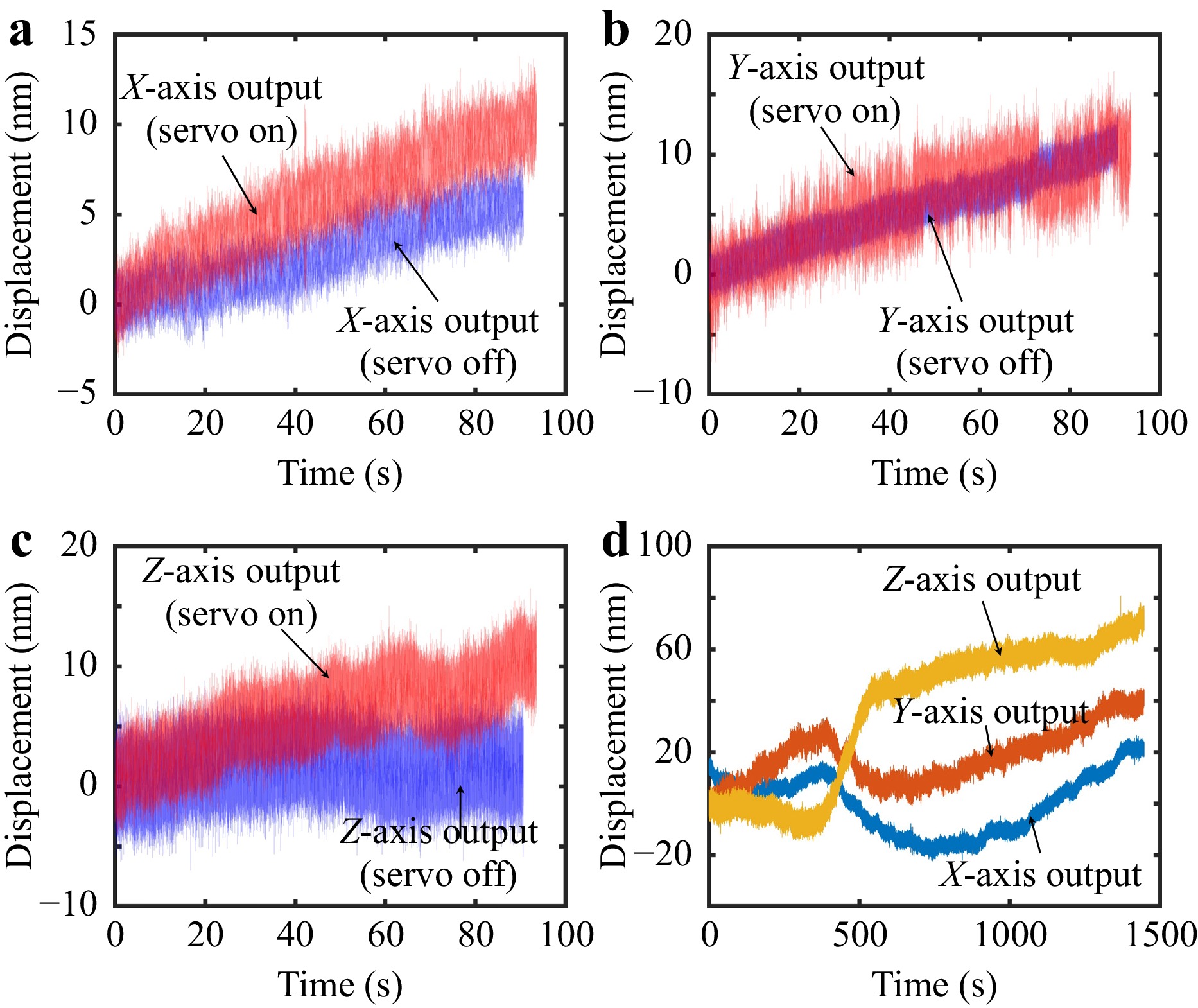
Fig. 8  Stability test. a X-axis open-loop and closed-loop stability over 90 s. b Y-axis open-loop and closed-loop stability over 90 s. c Z-axis openloop and closed-loop stability over 90 s. d XYZ-axes closed-loop stability over 1400 s.

(4) Repeatability: Repeatability refers to the consistency of measurement results in repeated tests under the same conditions. In this section, a large number of tests and evaluations were conducted for the XYZ axes. As shown in Fig. 9, box plots are used to statistically quantify the dispersion of 50 repeated tests with step displacements of 50 nm, 100 nm, 500 nm, and 1000 nm (speed: 1000 nm/s). Box plots display the median, interquartile range (IQR), and outliers, making them effective for assessing measurement stability under random noise.

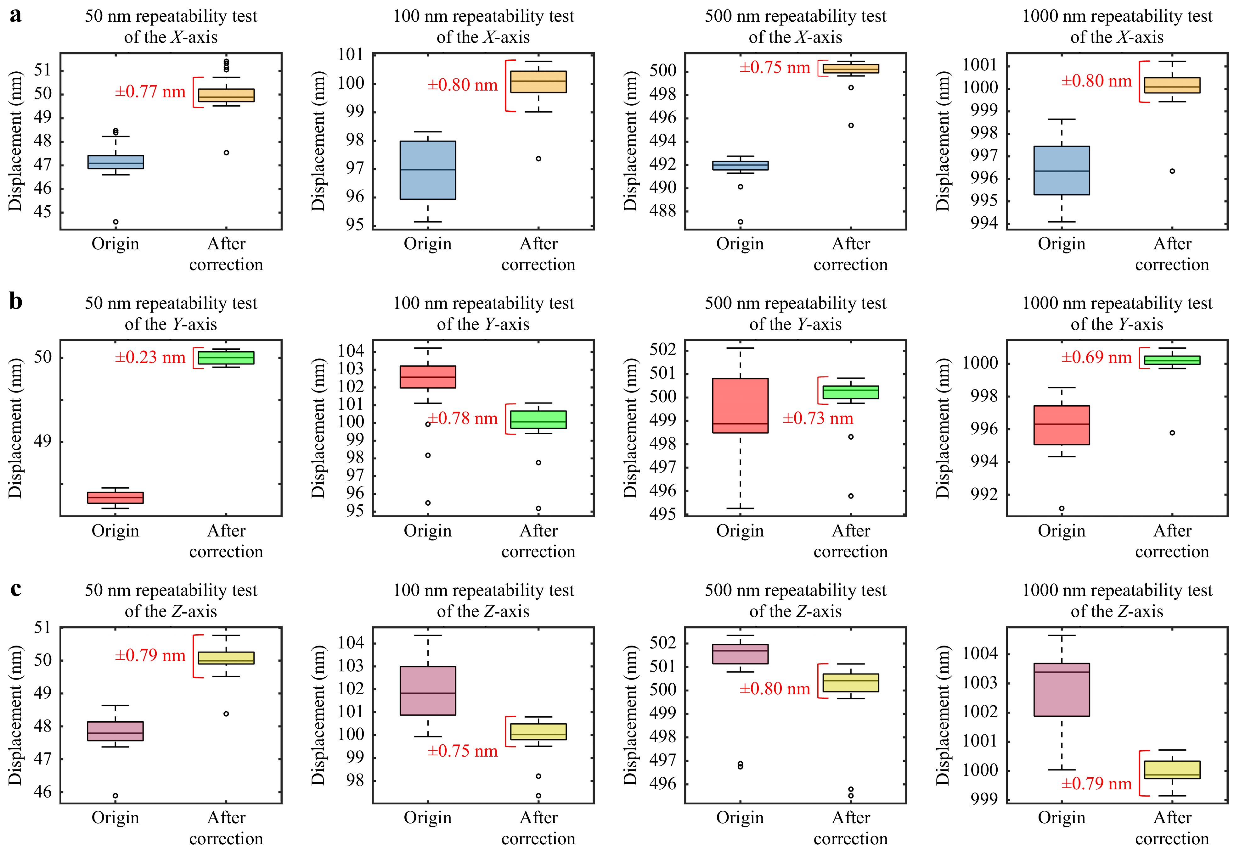
Fig. 9  Repeatability test. a X-axis. b Y-axis. c Z-axis.

To isolate the repeatability of the system from external influences (such as grating surface topography changes and assembly errors), the raw data were processed using cosine error correction. The corrected results (Fig. 9, “After correction” box) reflect the repeatability of the interferometer system. The following conclusions can be drawn from the figure: X-axis (Fig. 9a): All step sizes show IQR boundaries within ±0.8 nm, demonstrating excellent repeatability across various step sizes. Y/Z axes (Fig. 9b, c): Similar performance was observed, with IQR limits within ±0.8 nm and outlier density comparable to the X-axis.

Overall, the system achieves repeatability of 0.8 nm ($ 3 \sigma $) across all axes for a 1000 nm step. This performance is attributed to the zero dead-zone design, which eliminates random noise.

(5) Measurement range: The measurement range is a critical parameter of the measurement system, directly influencing its applicability in various scenarios. In this section, we use a 2D reflective grating with a period of 1000 nm as the measurement grating and the Newport HXP50-MECA as the displacement stage. As illustrated in Fig. 10a, the grating with dimensions of 15 × 15 × 5 mm³, is integral to the precise measurement of displacement along the XYZ axes. The system’s performance is validated by comparing experimental results with theoretical predictions, as shown in Fig. 10b-d. These figures show the displacement measurements along the X, Y, and Z axes, respectively, with the residuals indicating the difference between the measured and theoretical values. The measurement range of XYZ axes are 10 mm, 10 mm, and 2 mm, respectively. It is worth noting that the measurement range of the XY axis is primarily limited by the grating area. A larger grating area results in a larger measurement range, which could theoretically extend to the meter scale. Additionally, advanced methods for preparing large-area gratings have been proposed^{41, 42}. In the X-axis test (Fig. 10b), the maximum residual is 2.922 µm, and the minimum residual is −3.247 µm. For the Y-axis (Fig. 10c), the maximum residual reaches 1.868 µm, and the minimum residual is −3.251 µm. Finally, in the Z-axis test (Fig. 10d), the residuals range from 0.838 µm (maximum) to −0.820 µm (minimum). These residuals reflect a combination of errors from the measurement system and the displacement table motion. Overall, these residuals highlight the high precision of the system, confirming its capability for accurate 3-DOF displacement measurements.

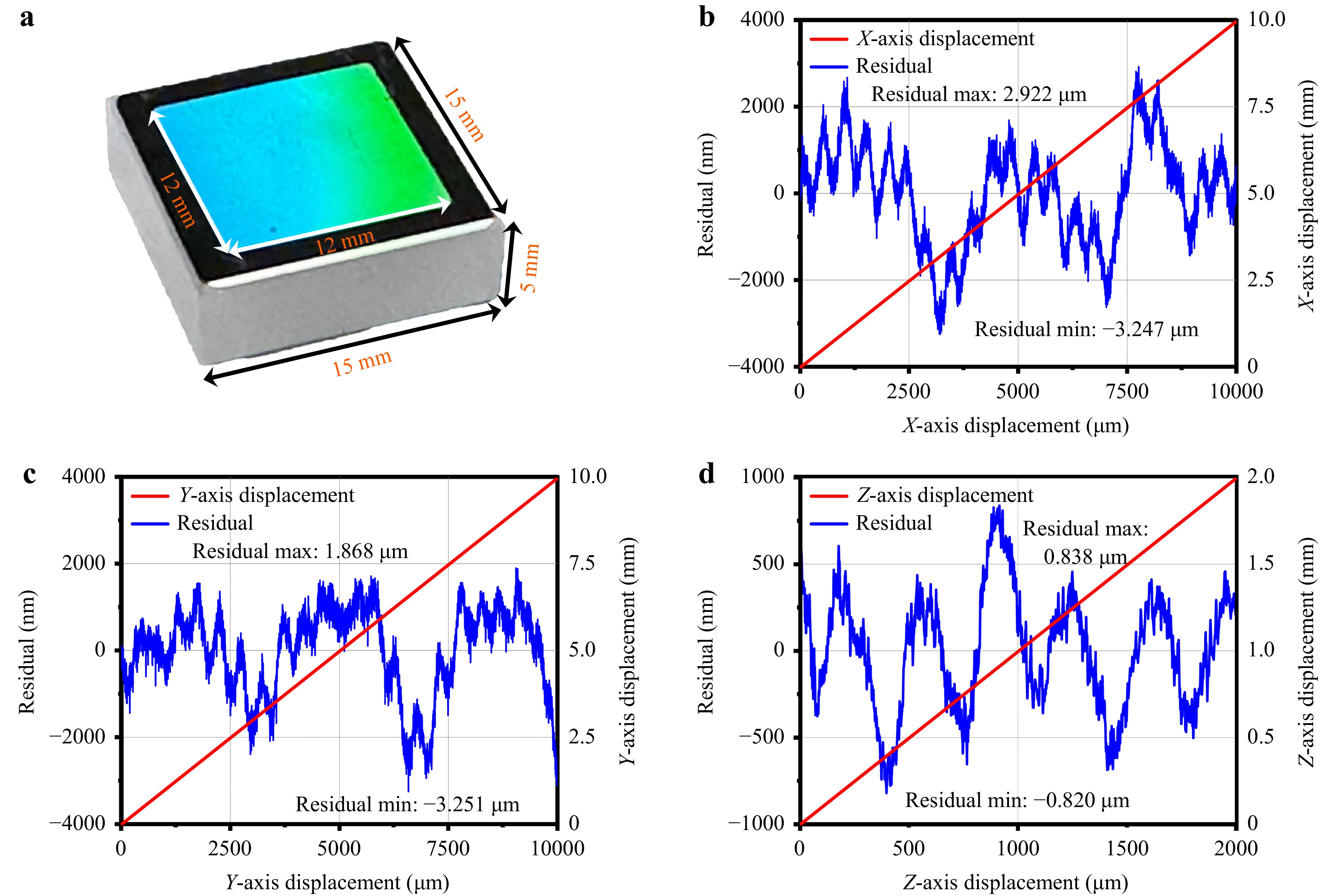
Fig. 10  Measurement range test. a Measuring grating and its dimension. b Test of X-axis measurement range. c Test of Y-axis measurement range. d Test of Z-axis measurement range.

(6) Summary: A summary of the proposed system’s performance indicators, resolution, linearity, repeatability, stability, and measurement range can be found in the last row of Table 1.

In a high-precision 3-DOF grating interferometry measurement system (M) integrated with a 3-DOF displacement stage (S), crosstalk errors emerge across multiple stages, significantly degrading measurement accuracy. As summarized in Table 2, crosstalk errors are primarily categorized into three types, which are introduced in detail below. Type-I: intrinsic crosstalk within the measurement system M arises from imperfect axis-decoupling in the computational model. To illustrate, nonlinear coordinate transformations or miscalibrated Jacobian matrices in the interferometric signal processing can induce cross-axis coupling, manifesting as nonlinear deviations that are proportional to multi-axis displacements. Type-II: installation-induced crosstalk arises from misalignment between the measurement system M and stage S, such as non-orthogonal mounting angles or tilts. This results in affine transformations in the measured data, often manifested as unintended linear slopes or offsets in the displacement curves. Type-III: stage-inherent crosstalk originates from mechanical and control coupling of axes of the stage S. Dynamic interactions such as periodic vibrations from ball screw harmonics or electromagnetic interference between servo drivers can propagate across axes, introducing sinusoidal artifacts in the interferometry readings. These cascading crosstalk effects highlight the need for systematic error isolation and compensation to ensure sub-micron precision in multi-axis metrology.

In the proposed system, for the Type-I error, crosstalk suppression begins with eliminating intrinsic algorithmic coupling. As demonstrated by Eq. 3, the axis-decoupling model establishes theoretical independence among the measurement axes, thereby nullifying Type-I crosstalk errors. Consequently, the subsequent analysis primarily concentrates on Type-II and Type-III crosstalk effects. Fig. 11a illustrates the system configuration, highlighting how motion along one axis (e.g., X-axis) can induce crosstalk in another (e.g., Z-axis). Fig. 11b quantifies this effect: when S remains stationary along the Z-axis, only minimal error fluctuations are observed. However, during X-axis motion, the Z-axis output exhibits a superimposed linear slope (Type-II, attributed to affine distortions from mounting misalignment) and a sinusoidal fluctuation (Type-III, caused by periodic mechanical coupling within S). In the following subsections, we propose a compensation method for both Type-II and Type-III errors.

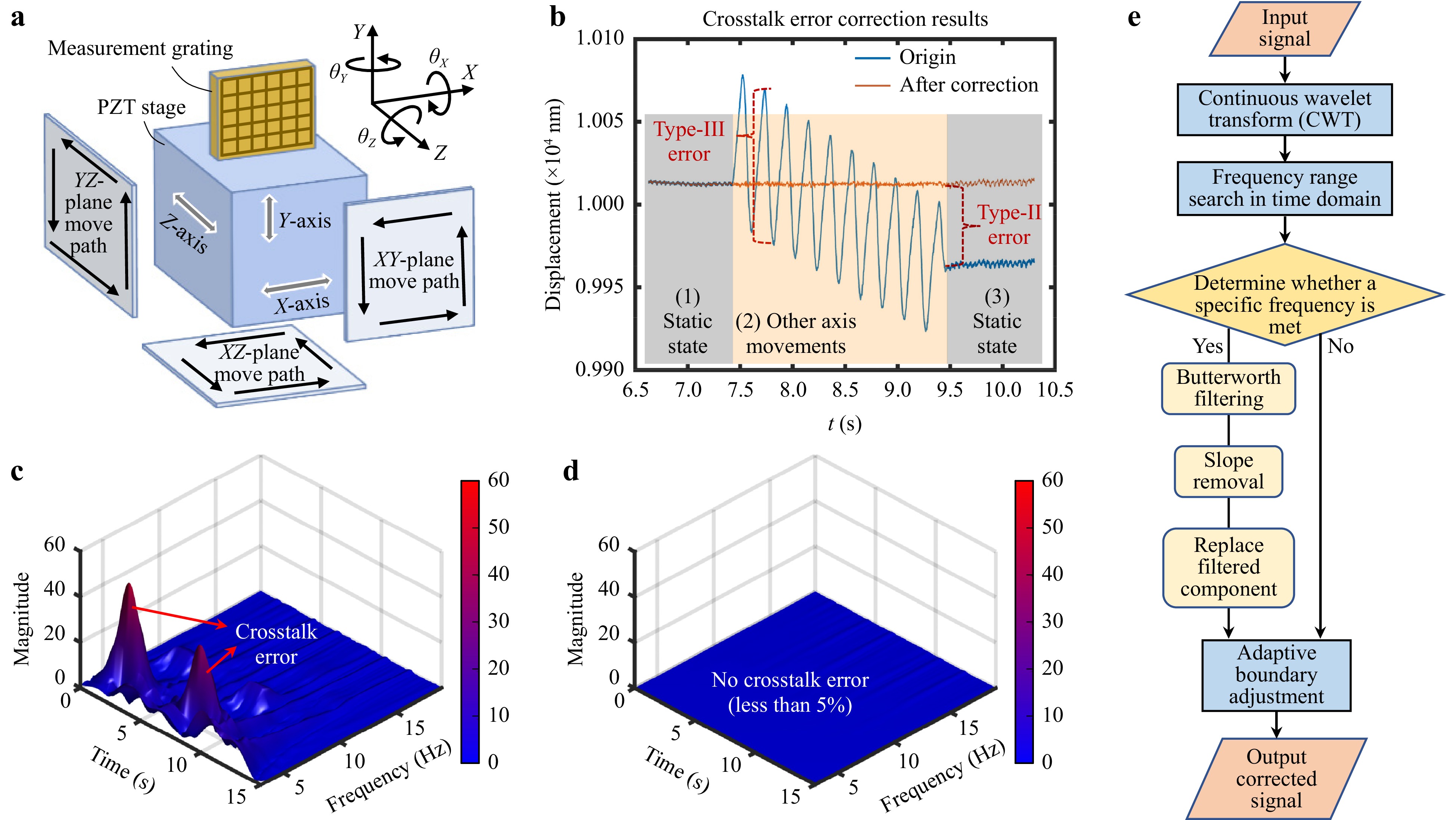
Fig. 11  Multi axes crosstalk error analysis and correction method. a Motion path of the grating in different planes. b In the XY plane, X-axis motion induces crosstalk error in the Y axis. c Wavelet transform diagram showing crosstalk error. d Wavelet transform diagram of crosstalk error after algorithm correction. e Flowchart of the correction algorithm.

Fig. 11c, d present the wavelet transform analysis of crosstalk errors before and after correction. The analysis reveals pronounced high-frequency components associated with crosstalk in Fig. 11c, whereas Fig. 11d illustrates the absence of significant crosstalk errors after correction, and the error is reduced to less than 5%. This demonstrates that the correction algorithm effectively detects and mitigates crosstalk errors, thereby enhancing measurement precision. The correction algorithm flowchart in Fig. 11e outlines the systematic approach to reduce crosstalk errors to below 5%. The process begins with a continuous wavelet transform (CWT) of the input signal, followed by a frequency range search within the time domain. If a specific frequency criterion is satisfied, the algorithm applies Butterworth filtering, removes any linear slope, and replaces the filtered components. Finally, adaptive boundary adjustments are performed to generate the corrected signal. This structured methodology enables effective suppression of crosstalk errors, thereby significantly enhancing the reliability of the measurement system. In conclusion, the implementation of the correction algorithm improves the system’s precision and long-term stability.

In this paper, we present the development of a novel heterodyne grating interferometer designed to meet the precise measurement requirements of next-generation high-end lithography systems and large-scale atomic-level manufacturing. This innovative approach features a zero dead-zone design, enhancing both performance and compactness, with overall dimensions of 90 × 90 × 40 mm³. The system achieves exceptional resolution, with 0.25 nm in the XY-axis and 0.3 nm in the Z-axis. Furthermore, linearity is maintained at superior levels, with performance metrics of 6.9 × 10⁻⁵, 8.1 × 10⁻⁵ and 16.2 × 10⁻⁵ for the X, Y, and Z axes, respectively. The repeatability of measurements has been validated, with results exceeding 0.8 nm@1000 nm, 0.69 nm@1000 nm, and 0.79 nm@1000 nm in the X, Y, and Z axes, respectively. Notably, the system’s stability is better than 20 nm in the XY-axis and 60 nm in the Z-axis after a 1000 s test. In addition, the measurement range of the XYZ axes of the measurement system is 10 mm, 10 mm, and 2 mm, respectively. When a larger grating is employed, the in-plane measurement range can be extended.

Comparative analyses with representative measurement systems from both industry and academia, as detailed in Table 1, reveal that the proposed method shows superior competitiveness in terms of integration, multidimensional capabilities, resolution, linearity, repeatability, and stability. This advancement highlights significant potential for ultra-high precision measurement applications. However, there are some limitations, primarily the limited measurement range of the Z-axis and the need for further development of the diffraction light collimation module, which will be addressed in subsequent work.

This research is supported by National Natural Science Foundation of China (NO. 62275142), Shenzhen Stability Support Program Project (NO. WDZC 20231124201906001) and Guangdong Basic and Applied Research Fund (NO. 2021B1515120007).