Bimodal tissue differentiation using hyperspectral imaging and elastographic Fourier transform profilometry

One of the most common cancer types worldwide in women is breast cancer¹. To ensure the complete surgical resection of the tumor, knowledge of the tumor boundaries is necessary. In addition to conventional frozen section diagnostics, new intraoperative diagnostic methods are being used, which offer reduction of the patient’s operation time or the need for further resection and enable tissue-preserving surgeries. Some of these techniques, like multispectral imaging (MSI), could either be used to recognize tissue differences during surgery or during pathological analysis.

Using spectral signatures of tissue is a well-established technique for tissue differentiation in medicine. A common method is fluorescence imaging with fluorescence markers like indocyanine green (ICG), which is for example used in lymph node detection^2–5. The fluorescence signal of the tissue labelled with ICG is imaged in the near infrared (NIR) by an additional monochromatic image that is superimposed on the normal red-green-blue (RGB) image⁵. In addition to chromophore characteristics, differences in the vibrational states of molecules can also be determined spectroscopically. Raman spectroscopy can be used to detect epigenetic changes by measuring inelastic scattering effects and thus contribute to tissue differentiation^6–10. Another method of MSI is narrow-band imaging, in which the tissue is illuminated with blue and green light. Unlike red light, these wavelengths do not penetrate as deeply into the tissue and are primarily absorbed by vascular structures. Hence, the contrast of these structures, like blood vessels, capillaries or mucosa is increased and becomes more visible^11–13.

Hyperspectral imaging (HSI) differs from MSI by the number of spectral channels¹⁴. While MSI uses a few spectral channels, HSI usually analyzes more than 30. There are different ways to implement such an HSI setup, ranging from line spectrometers to HSI snapshot cameras. The latter use special camera sensors including interference filters for spectral filtering¹⁵. In the context of medical technology, there are already different variants of multi- and hyperspectral laboratory setups, which are for example used for perfusion analyzes or tissue differentiation^14,16–22. In recent years, two medically approved HSI devices have also been developed, which can be used either as a larger camera unit for open surgery or endoscopically for minimally invasive procedures (Tivita Tissue and Tivita Mini, Diaspective Vision)^20,23.

On the other hand, differentiating tissue types based on their elastic properties is another common method widely used, especially in the early detection of breast cancer^24–26 and in open surgery, where the surgical staff estimates the boundaries of the malignancies via palpation^27–29. This is attributed to the fact that tumor tissue exhibits a greater stiffness compared to the surrounding normal tissue types³⁰. As minimally invasive surgery (MIS) becomes increasingly common due to its numerous advantages for patients, such as smaller incisions and consequently shorter recovery times, the development of a potentially miniaturizable sensor concept should be pursued. However, the tissue’s stiffness cannot be exploited as the haptic feedback is reduced in MIS and lacking in robot-assisted surgery^31,32. Minimally invasive elastographic measurement techniques are therefore currently both under development or already in clinical practice, like ultrasound elastography^33,34, optical coherence elastography^35,36 or water flow elastography^37,38. These techniques, however, have their limitations, for example being only point or contact-based measurements, or low in spatial resolution. Recently, a miniaturized endoscopic measurement setup based on Fourier transform profilometry (FTP) has been developed, which has been described and validated in previous publications^39–42. As a fiber-based method it offers the potential for fast, full-field, and contact-free elastographic measurements, making it highly suitable for dynamic settings. Furthermore, it offers the additional advantage of being easily integrable alongside camera-based imaging modalities, such as HSI systems.

In this work, we therefore present a novel multimodal imaging system that combines spectral and elastographic information to differentiate between altered and healthy tissue.

The proposed multimodal sensor system consists of two separate illumination subsystems, which create the bimodality and a single imaging path for combined measurements. We first introduce the individual modalities and describe the combined system. Then, we outline the general measurement procedure, followed by the measurement routines of the individual systems as well as their preprocessing and evaluation methods.

The full schematic and the laboratory setup is shown in Fig. 1. The used HSI system is designed as a monochromatically scanning setup. It consists of a halogen light source (Thorlabs OSL2IR) to provide a broad spectral range, which is coupled through a fiber bundle (Thorlabs OSL2FB) to a customized monochromator (entrance aperture diameter 1 mm, rotatable grating (Thorlabs GR25-0608), filterwheel (Thorlabs FW102C) with longpass filters (Thorlabs FELH0400, FELH0550 and FELH0900) and two lenses for collimation and imaging with 100 mm and 120 mm focal length) to split the broadband input spectrum into narrow spectral bands. The light is then coupled into a multimode fan-out fiber bundle (Thorlabs BFL44LS01, orientation of fiber cores: vertical), where the core diameters of each fiber serve as the monochromator’s exit apertures, to illuminate the tissue surface. The imaging part of the setup consists of an achromatic doublet as the objective, a dichroic mirror (Thorlabs DMSP950T) and two monochrome cameras, one for the visible (VIS) and NIR (Ximea MQ013MG-E2) and one for the short wave infrared (SWIR) range (Raptor Photonics Ninox 640 SU), each equipped with an objective lens (VIS/NIR: Edmund Optics #67-714, SWIR: Computar ViSWIR Lite M1614-VSW). The dichroic mirror splits the light according to its spectrum, so that it can be imaged with the corresponding camera, either the VIS/NIR for $ \lambda $ < 950 nm or the SWIR camera for $ \lambda \geqslant $ 950 nm. The measurement setup, including monochromator and acquisition of both cameras, is automatically controlled via a Python script using the measurement software itom^43,44.

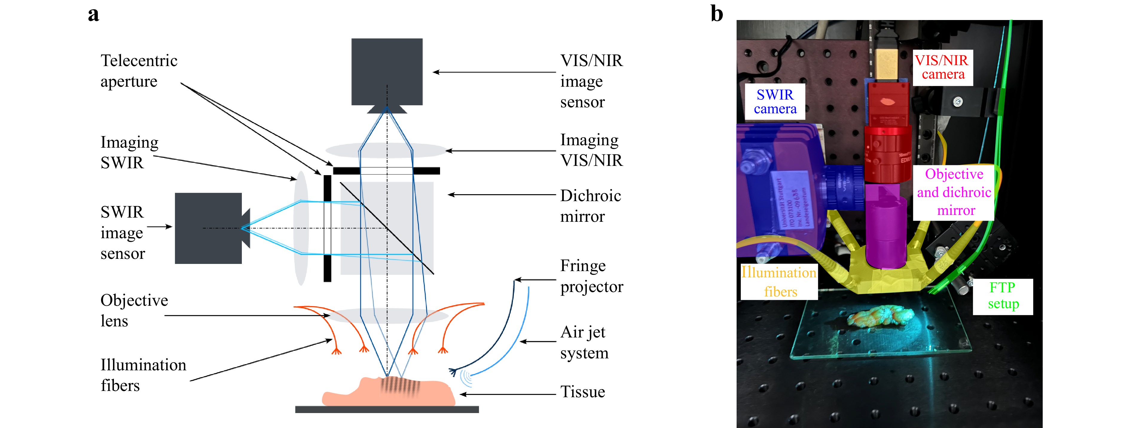
Fig. 1  Schematic a and laboratory setup b. The HSI setup consists of the illumination fibers (yellow), the objective and dichroic mirror (purple) and the two camera systems (red and blue). The elastographic FTP setup is added on the right and consists of the air jet system and fringe projector (green), the objective and the dichroic mirror (purple), and the VIS camera system (red).

The characterization results show a good lateral resolution (VIS/NIR: approximately 22 µm, SWIR: approximately 56 µm) and a high signal to noise ratio. To measure the tissue reflectance spectra, the illumination spectrum was iterated from 450 nm to 1450 nm in 10 nm steps, resulting in 101 spectral channels with a mean spectral resolution of $ \left\langle{{FWHM}_{\rm{vis,nir}}}\right\rangle $ = 12.53 ± 0.59 nm (full width at half maximum) for the VIS/NIR and $ \left\langle{{FWHM}_{\rm{swir}}}\right\rangle $ = 9.1 ± 2.93 nm for the SWIR⁴⁵.

The aforementioned fiber-based elastographic fringe projection setup is integrated to the HSI part by placing it at a triangulation angle next to the optical axis of the VIS camera. The projection part of the setup consists of a 3D-printed miniaturized fringe projection lens (Printoptix GmbH, Pat. No. DE102023115518A1)⁴⁶ mounted onto the tip of an optical fiber (Thorlabs M113L02). The fiber is illuminated using a fiber-coupled LED light source (Thorlabs M625F2) emitting light at a peak wavelength of $ \lambda $ = 625 nm. This wavelength was chosen as the reflectance spectrum for healthy breast tissue using diffuse reflectance spectroscopy rapidly increases close to its maximum for $ \lambda $ > 600 nm and remains near constant over a broad wavelength range^47–51. Consequently, breast tissue allows for better visibility of the fringe pattern for these wavelengths.

A cystoscopic needle (Cook Medical G14220, 090001) connected to a pressurized air valve is mounted next to the fringe projection fiber to indent the tissue using an air jet impulse. The solenoid valve (Landefeld M 314 24V) is controlled automatically using a microcontroller and the air pressure manually by a pressure regulator (Landefeld FDR 03-7-14).

The measurements were performed at the Department of Gynecology and Obstetrics of the University Hospital Tübingen in accordance with "The Code of Ethics of the World Medical Association" (Declaration of Helsinki) and approved by the Ethics Committee of the University of Tübingen (UKT IRB# 440/2023/BO2). Patients were enrolled in the study after providing informed consent. This study is part of a general tissue differentiation study, testing several new measurement concepts as part of the Research Training Group 2543. As the measurement principles shown here did not measure all patients in the general study, only a subset of four patients measured by both HSI and FTP is considered below.

The patients in this study were aged between 37 and 61 years and were clinically diagnosed with cT1, cT2 or cT3 breast tumors. Half of the group was treated with neoadjuvant hormone therapy.

After surgical resection of the tumor, the native tissue was analyzed first and cut into lamellas by a pathologist. One of the tumor lamellas was then placed onto a sample plate and then passed to the sensor system (see Fig. 1b). For each sample, a presumed tumor and healthy area of the lamella was measured with each modality. Fig. 2 shows the raw breast tissue of each patient. The measurement positions are color-coded in dark blue for tumor and light blue for healthy tissue. One healthy presumed measurement position of patient #26 was diagnosed with a precursor lesion of type Ductal Carcinoma in Situ (DCIS) in the histopathological examination afterwards (green circle). Due to the limited comparative data on precursor lesions like DCIS, we will not consider this as part of this work.

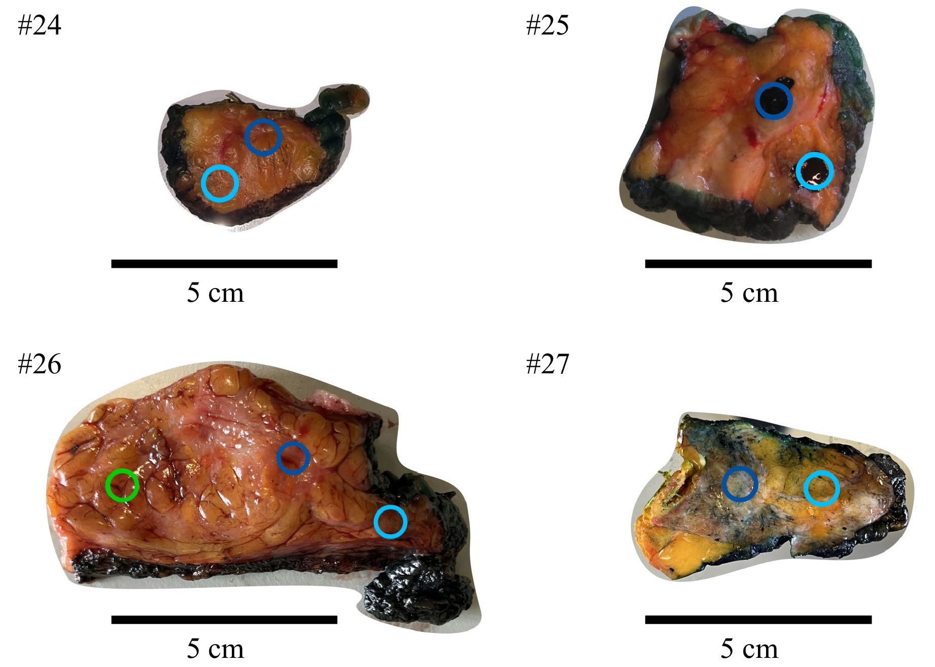
Fig. 2  Examined tissues with highlighted measurement positions (circles). Dark blue: Tumor, light blue: Healthy, green: Precursor lesions. The images of patients #24 and #27 show the tissues before measurement. The upper right image shows the tissue of patient #25 after finishing the measurements, indicated by the already applied pathological dye. Patient #26 was measured at three different positions. As can be seen by the green colored circle, the measurement position was presumed healthy but was diagnosed containing DCIS during histopathological examination and was thus disregarded for further analysis.

The measurement order was HSI followed by elastographic FTP measurements. After finishing the measurements, the measurement areas were marked with pathological dyes (see Fig. 2, #25), to garantuee a local pathological analysis for each of the measurement positions. The lamella was then returned to the pathology for further processing and histopathological analysis.

To ensure the optimal object distance for each spectral channel of the hyperspectral as well as for the elastographic system, a focus referencing measurement is performed first. For this purpose, a separate laser line was projected onto the tissue surface. The vertical stage was then moved, so that the object distance sweeps through the focal position. By measuring the line thickness over the current object distance, the focus position can be indicated by the minimum of the measured line thickness.

For the measurements themselves, the illumination spectrum was iterated over the spectral range of the system and for each spectral channel an image was taken, resulting in two hyperspectral cubes, one for VIS/NIR and one for SWIR. To demonstrate the reproducibility and evaluate the influence of noise, five individual cubes were recorded for each measurement area.

To analyze the spectral information gained by the measurements, at first the influence of the varying exposure time $ {t}_{\exp} $ per spectral channel to the raw intensity of the object $ {I}_{\rm{obj,raw}} $ is corrected via Eq. 1.

Subsequently, dark and white corrections are applied to reduce noise and to account for the camera sensor’s sensitivity across each spectral channel. According to Eq. 2, the dark correction is performed by subtracting the exposure time corrected intensity of a dark image $ {I}_{\mathrm{d}\mathrm{a}\mathrm{r}\mathrm{k},\mathrm{e}\mathrm{x}\mathrm{p},\mathrm{c}\mathrm{o}\mathrm{r}\mathrm{r}} $ obtained by measuring a highly absorbing foil (Edmund Optics, #12-695 Acktar Metal Velvet Foil).

To correct the influence of the camera sensor’s sensitivity, the dark corrected image intensity $ {I}_{\mathrm{o}\mathrm{b}\mathrm{j},\mathrm{d}\mathrm{a}\mathrm{r}\mathrm{k},\mathrm{c}\mathrm{o}\mathrm{r}\mathrm{r}} $ is then divided by a dark corrected white image intensity $ {I}_{\mathrm{w}\mathrm{h}\mathrm{i}\mathrm{t}\mathrm{e},\mathrm{d}\mathrm{a}\mathrm{r}\mathrm{k},\mathrm{c}\mathrm{o}\mathrm{r}\mathrm{r}} $, where the white image is obtained by measuring a spectralon. This results in the final intensity $ {I}_{\mathrm{o}\mathrm{b}\mathrm{j},\mathrm{s}\mathrm{e}\mathrm{n}\mathrm{s},\mathrm{c}\mathrm{o}\mathrm{r}\mathrm{r}} $.

After preprocessing, the visible and near-infrared cubes are combined by aligning the two camera coordinate systems. To reduce intensity variations due to object distance variations caused by the surface topology, a min-max normalization of each image pixel is performed according to its spectral axis. The final spectra can then be extracted pixel-wise.

For profilometric measurements, the tissue was illuminated by the projected fringe pattern. A fixed exposure time $ {t}_{\exp} $ was then set to achieve an appropriate balance between image intensity and a reduced amount of over-exposed pixels due to specular reflections. In order to record the time-dependent viscoelastic behavior of the tissue, a series of images is taken over $ {t}_{\rm{meas}} $ = 20 s for each of the five individual measurements. The number of images taken per series $ {n}_{\mathrm{i}\mathrm{m}\mathrm{g}} $ results from the measurement and exposure time via Eq. 4.

The pressurized air valve was opened for five seconds during this time period so that the tissue surface can be recorded for five seconds before, five seconds during and the remaining time after the indentation force was applied.

The temporal indentation was evaluated using standard FTP^52–54. The fringe images are first transformed to the spatial frequency domain (SFD) using a 2D Fourier transform (FT). A bandpass filter is used to manually select the carrier frequency component, which is then shifted to the origin of the SFD. A Gaussian blur is used on the filtering window to mitigate the Gibbs effect. The size of the Gaussian kernel was chosen to be the next nearest odd integer of the filtering window size. For the standard deviations of the Gaussian kernel $ \sigma $, the size of the filtering window was treated as its FWHM, so that $ \sigma $ can be calculated via Eq. 5.

Then, an inverse FT of the carrier frequency component is applied to determine the phase angle $ \phi $ at every pixel of the image. The 2$ \pi $-wrapped phase is then unwrapped using the phase unwrapping algorithm by Lei et al.⁵⁵. The first phase image in the image stack, which represents the non-deformed surface, is subtracted from every other phase image to determine the temporal indentation independent of the measured surface profile. The temporal viscoelastic deformation behavior can then be obtained by evaluating one or multiple pixels along the image stack.

In the following, we present the measurement results both individually and in combination. To demonstrate the suitability of the individual sensor systems for tissue differentiation, we initially perform a qualitative and quantitative analysis. The results include spectral and elastographic data from the presumed tumor or healthy tissue, which are subsequently classified as either tumor or healthy by the pathology department based on the histopathological findings. Furthermore, we show how each of the individual systems benefits from the combination in the overall bimodal system.

Five HSI cubes are acquired per patient to analyze the influence of temporal noise. Therefore, the mean value and the corresponding standard deviation are calculated for each pixel of each spectral channel, resulting in a mean HSI cube per tissue type. Fig. 3 shows the influence of temporal and spatial averaging by comparing the mean spectrum of a single pixel over several measurements (green) and the mean spectrum of a spatial region of interest (ROI, blue) of a single measurement. The top images show presumed healthy tissue (light blue) and the bottom images show presumed tumor tissue (dark blue). For better visualization of the evaluated pixel, a camera image at $ \lambda $ = 620 nm is shown, in which the ROI and the pixel for temporal averaging are highlighted. The low standard deviation of temporal averaging indicates that the variability among the single measurements has minimal impact on the spectrum of a single pixel. In contrast, the spatial averaging over 60 × 80 pixels, which represents approximately 1 × 1.3 mm in object space, shows a larger variance. This is to be expected as averaging over many pixels can potentially lead to averaging over different tissue components. Because of this behavior, only the standard deviation of spatial averaging is shown in the following figures.

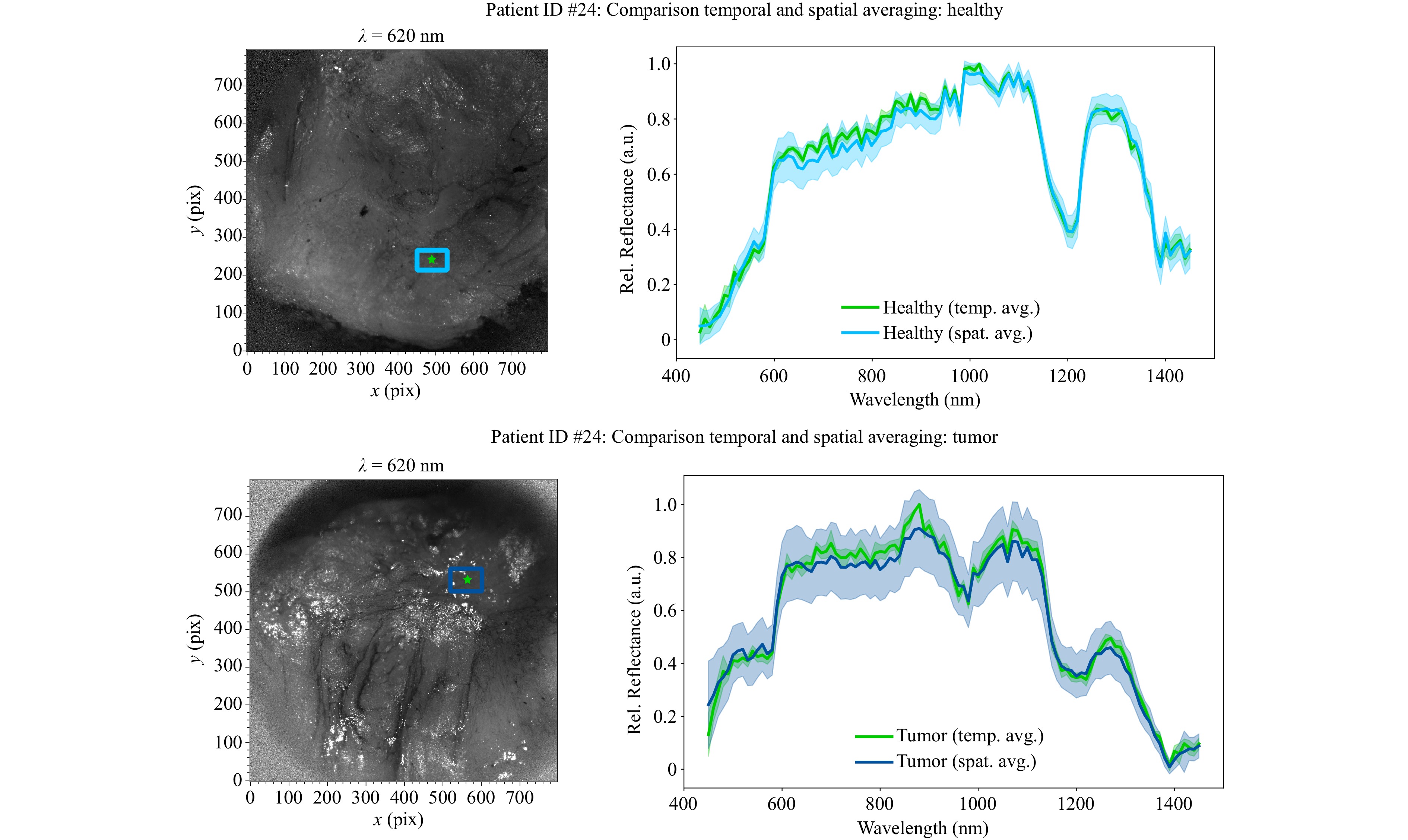
Fig. 3  Comparison of temporal and spatial averaging of HSI measurements. Left: Camera image of tissue surface. The ROI for spatial averaging is marked in blue, the single pixel for evaluating the averaging over five individual cubes is marked in green. Right: The tissue spectra with the corresponding standard deviations shown as shaded areas, blue for spatial averaging and green for temporal averaging. Both assumed tissue types were confirmed in the subsequent histopathological examination.

By combining the temporal and spatial averaged spectra of healthy and tumor tissue in one plot, the single tissue spectra can be compared more easily, see Fig. 4. It can be observed that there are distinct differences in the spectra. Red outlines have been added to emphasize these areas. For better generalizability of interesting and promising spectral channels for tissue differentiation, the final evaluation is done after averaging the results of each patient.

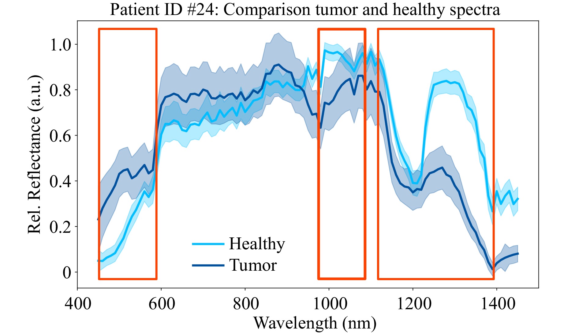
Fig. 4  Mean healthy (light blue) and tumor (dark blue) spectra of the two ROIs shown in Fig. 3. Potentially interesting parts of the spectrum for tissue differentiation are highlighted by red boxes. Both assumed tissue types were confirmed in the subsequent histopathological examination.

Fig. 5 shows the mean spectra and the corresponding standard deviation between all four patients. The spectra are obtained by computing a mean spectrum per patient and tissue type by using temporal and spatial averaging and subsequently calculating the mean over all patients. It can be seen that the previously identified areas of interest exhibit consistent characteristics even across multiple patients. Tumor tissue absorbs more in the SWIR but reflects more in the VIS regions, respectively. Additionally, the difference of reflectance at $ \lambda $ = 980 nm – 1080 nm is much higher for tumor than for healthy tissue, while the difference between $ \lambda $ = 1200 nm – 1250 nm is greater for healthy tissue. Furthermore, the width of the peak around $ \lambda $ = 1200 – 1300 nm is smaller for tumor in comparison to healthy tissue.

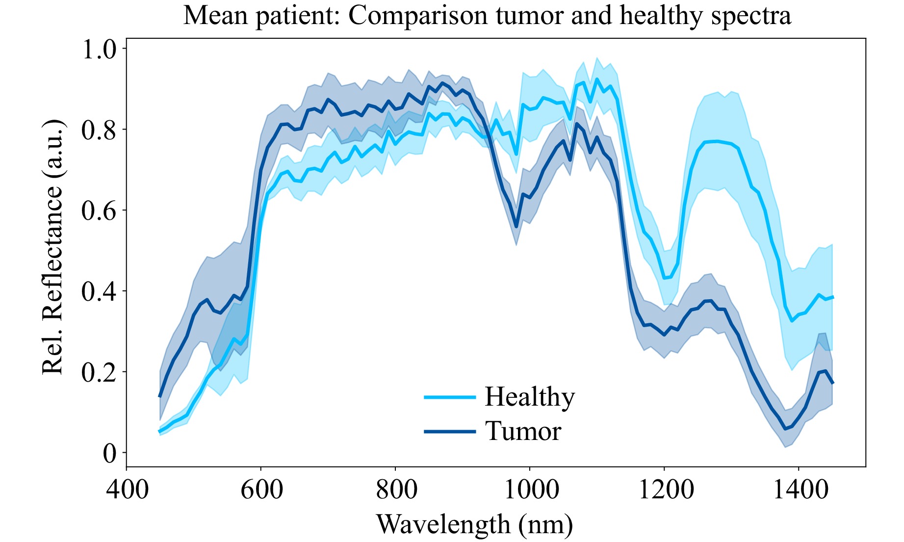
Fig. 5  Mean healthy (light blue) and tumor (dark blue) spectra of all measured patients with corresponding standard deviations between patients. All assumed tissue types were confirmed in the subsequent histopathological examination.

Fig. 6 shows the corrected mean normalized images of tumor tissue of patient #25 at the above mentioned interesting spectral ranges. As can be seen, the presumed tumor areas are well differentiable from the surrounding healthy tissue. However, the presumed tumor areas seem to have different dimensions in the VIS and SWIR range. Since the presumed tumor SWIR signatures are also partially visible in some of the images declared as presumed healthy, it is reasonable to assume that these are either not clear tumor components, but rather tissue types that occur in both tumor and healthy tissue, such as connective tissue.

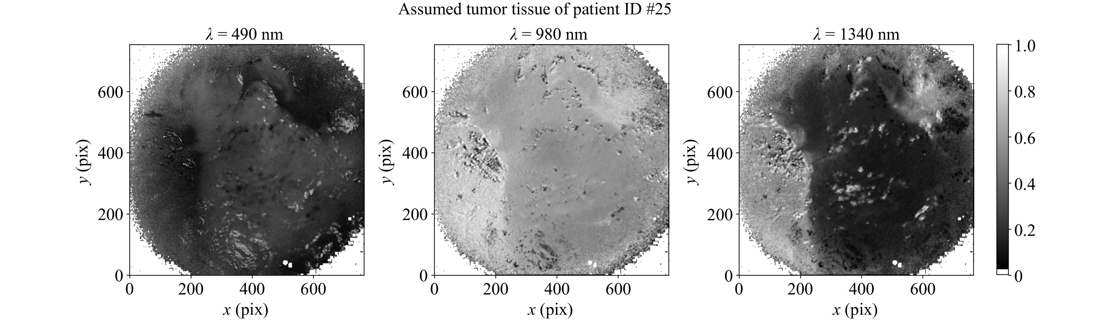
Fig. 6  Corrected mean normalized intensities for $ \lambda $ = 490, 980 and 1340 nm of patient #25. The assumed tumor can be seen by increased (left) or reduced reflectance (middle and right). The tumor assumption was confirmed in the subsequent histopathological examination.

This ambiguity of the SWIR spectral markers can be clarified by overlaying the histopathological slide with the HSI images. As can be seen in Fig. 7, the presumed tumor areas of patient #25 show a good match to the histopathological section. The fact that it does not fit perfectly can be explained by the further but necessary pathological treatment of the tissue and the resulting shrinkage, as well as by the fact that the HSI image shows the tissue surface, whereas the histopathological section shows a deeper cell layer due to the embedding procedure. Additionally, by overlaying camera images with the histopathological results, a pixel-wise mapping of the obtained spectra per tissue type can be achieved.

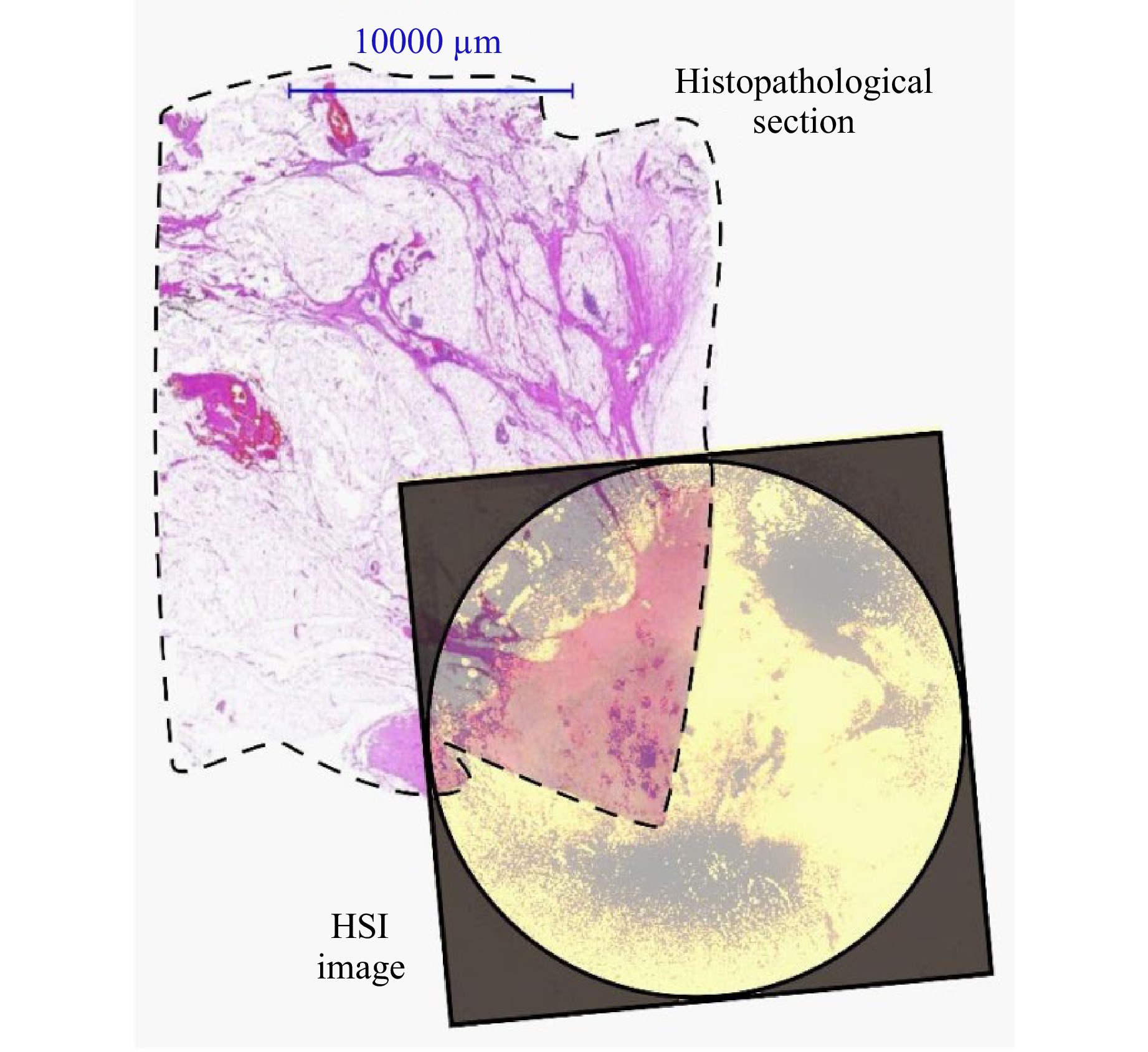
Fig. 7  Overlay of histopathological slide with HSI spectral channel at $ \lambda $ = 490 nm of patient #25. The dashed line highlights the border of the histopathological section. The border of the HSI image is highlighted by the camera aperture. For better visualization, the HSI image is contrast enhanced and colored. White areas of the histopathological slide represent healthy fatty tissue, while pink lines indicate septa. Reddish regions in the overlay area represents the tumor. Due to pathological limitations, the histopathological section does not cover the entire measurement range of the HSI image.

For quantitative analysis, a Support Vector Machine (SVM) for classification by scikit-learn⁵⁶ with a radial basis function kernel and standard default parameters is trained with the ROI spectral data of patients #24 to #26 and is tested with the ROI spectral data of patient #27. Table 1 shows an overview of the resulting training and test dataset.

This results in an accuracy of 83% and an F1-Score of 85%. The precision of the classification is 75%, 99% for the recall, and 67% for the specificity. Fig. 8 shows the corresponding confusion matrix.

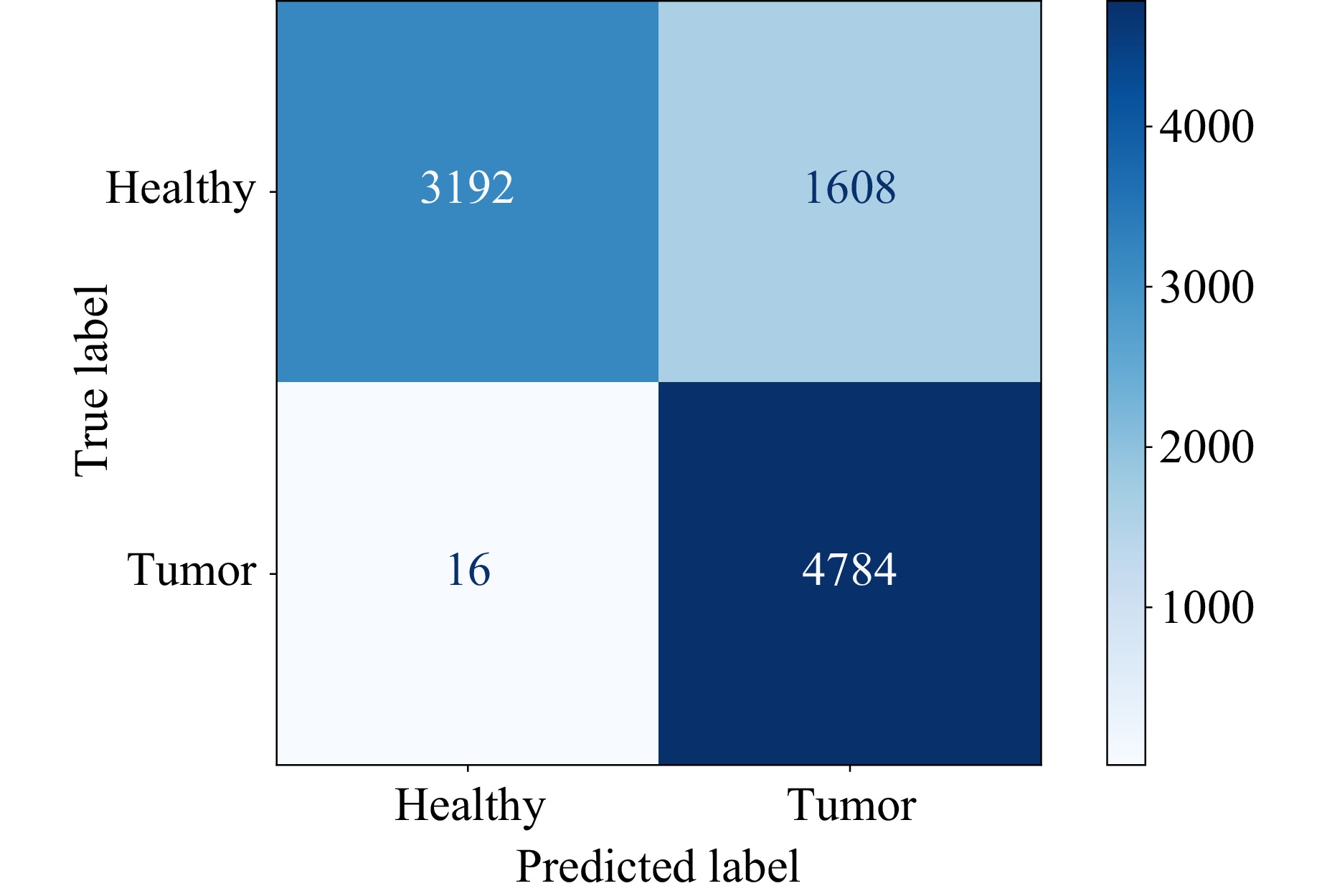
Fig. 8  Confusion matrix of SVM classification with parameters shown in Table 1.

Based on these initial measurements, it can be concluded that tissue differentiation based on spectral information in the visible to shortwave infrared spectral region is possible. In order to verify these spectral markers found, further measurements must be made that also take into account the different tissue types, such as connective tissue, special histological types of breast cancer, like lobular cancer, or precursor lesions, such as DCIS.

As with the HSI measurements, five elastographic FTP measurements were taken per patient to analyze the influence of temporal noise. The mean values and standard deviations are calculated for the same ROIs and in the same manner. Fig. 9 shows the average indentation depths of all five measurements in the same ROIs as shown in Fig. 3 next to their fringe images. The phase values of $ {n}_{\mathrm{i}\mathrm{m}\mathrm{g}} $ images are displayed evenly spaced within the time frame of $ {t}_{\mathrm{m}\mathrm{e}\mathrm{a}\mathrm{s}} $. The discrepancy between the plotted and the aforementioned indentation times is caused by the Python acquisition script experiencing a slow down during indentation due to the concurrent acquisition and indentation commands, which in turn extends the actual measurement time. The high standard deviation by the temporal averaging indicates that the variability of the reconstructed indentation depths on a single pixel among the measurements, especially for tumor tissue, has a substantial impact. In contrast to the HSI measurements, spatial averaging reduces this variability substantially, which can be explained by the fact that the air pressure force is uniformly distributed over a larger area, which causes the indentation to be also more uniform. The influence of temporal differences in phase values due to for example phase singularities in the reconstructions can thus be mitigated. Moreover, spatio-temporal averaging leads to a substantial reduction in variance of the measured indentation depths for all patients, which can be seen in Fig. 10. All indentation curves exhibit a consistent behavior characteristic of viscoelastic deformation.

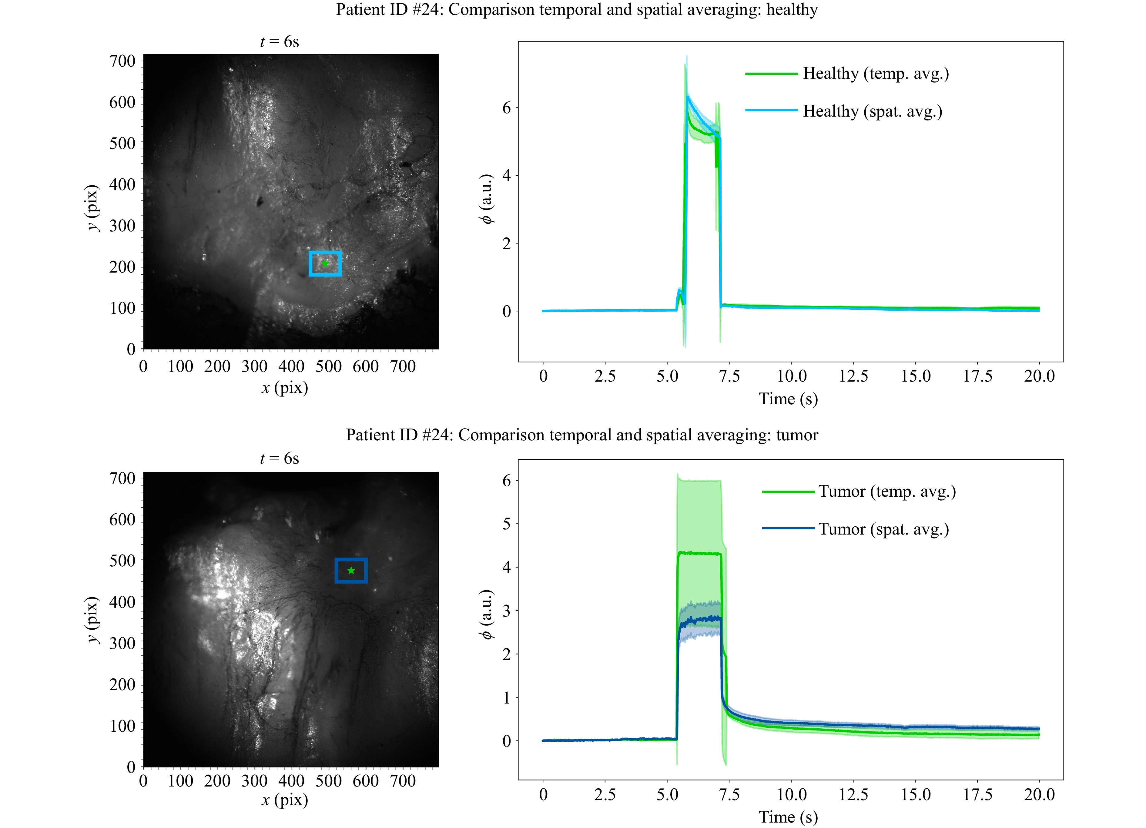
Fig. 9  Comparison of temporal and spatial averaging of FTP measurements. Left: Fringe image of tissue surface during elastographic indentation. The ROI for spatial averaging is marked in blue, the single pixel for evaluating the averaging over five individual image series is marked in green. Right: Mean tissue indentation depth as phase values with the corresponding standard deviations as shaded areas, blue for spatial averaging and green for temporal averaging. Both assumed tissue types were confirmed in the subsequent histopathological examination.

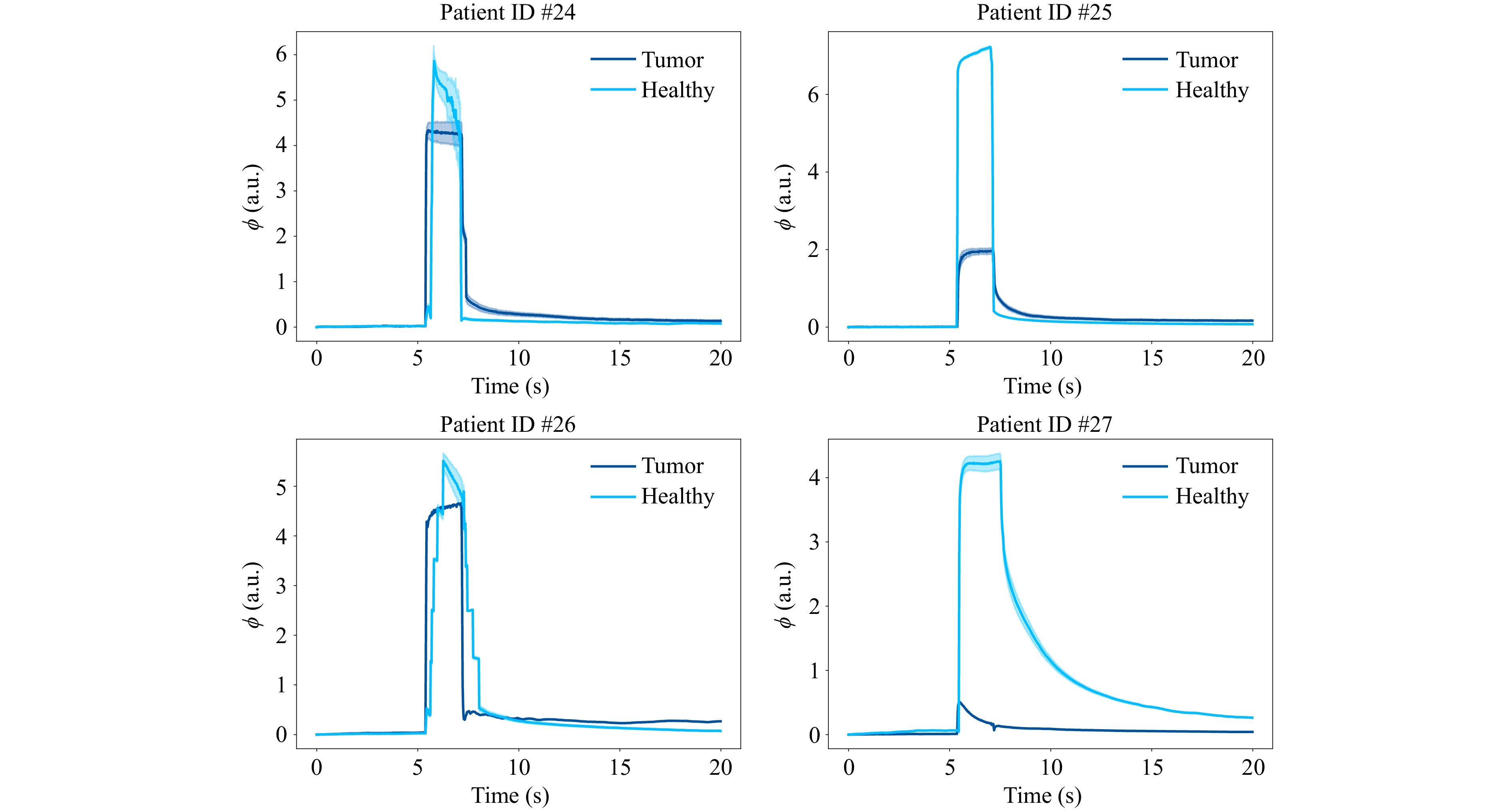
Fig. 10  Viscoelastic indentation curves of tumor and healthy tissues for all patients. All tissue types were confirmed by histopathological examination.

Differentiating tissue, for example by thresholding at the maximum of the average indentation of tumor tissue⁴² plus an integer multiple of its maximum standard deviation is possible in principle, especially for patients #25 and #27, although it can also be seen that for patients #24 and #26, the indentation depths between healthy and tumor tissue do not differ by much. Another way of setting a suitable threshold employed in this study mimicks a reference measurement based approach. First, the series of five healthy measurements are spatio-temporally averaged for the reference maximum indentation depth $ {\overline{\phi }}_{\mathrm{h},\mathrm{m}\mathrm{a}\mathrm{x}} $ (light blue curves in Fig. 10). Then, the maximum standard deviation $ {\sigma }_{\phi ,\mathrm{h},\mathrm{m}\mathrm{a}\mathrm{x}} $ of that average indentation time series (light blue shades in Fig. 10) is determined to calculate the reference threshold by setting $ {\phi }_{\mathrm{t}\mathrm{h}\mathrm{r}\mathrm{e}\mathrm{s}\mathrm{h}}={\overline{\phi }}_{\mathrm{h},\mathrm{m}\mathrm{a}\mathrm{x}}-2{\sigma }_{\phi ,\mathrm{h},\mathrm{m}\mathrm{a}\mathrm{x}} $. A binary classification can then be performed by comparing the maximum indentation depth of a presumed tumor tissue $ {\phi }_{\mathrm{t},\mathrm{m}\mathrm{a}\mathrm{x}} $ to the reference threshold $ {\phi }_{\mathrm{t}\mathrm{h}\mathrm{r}\mathrm{e}\mathrm{s}\mathrm{h}} $. The tissue pixel with the corresponding indentation will be assigned the label “healthy” if $ {\phi }_{\mathrm{t},\mathrm{m}\mathrm{a}\mathrm{x}}\geqslant {\phi }_{\mathrm{t}\mathrm{h}\mathrm{r}\mathrm{e}\mathrm{s}\mathrm{h}} $ and “tumor” if $ {\phi }_{\mathrm{t},\mathrm{m}\mathrm{a}\mathrm{x}} < {\phi }_{\mathrm{t}\mathrm{h}\mathrm{r}\mathrm{e}\mathrm{s}\mathrm{h}} $. Performing the differentiation over every pixel of true tumor ROIs used for the spatio-temporal averaging in every single measurement (96000 in total) yields 76800 correctly classified tumor pixels and 19200 falsely classified pixels. Hence, a precision of 80% can be achieved.

In contrast to the HSI system, no clear tumor boundary can be extracted by the phase map, since it produces only a depth map relative to the tissue’s surface at rest (see Fig. 11).

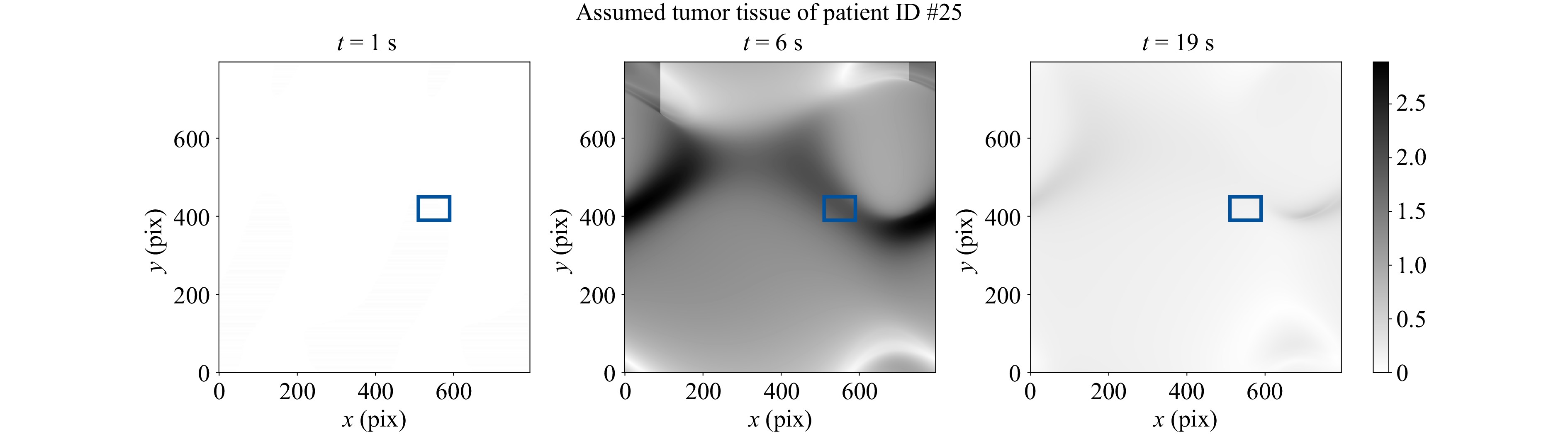
Fig. 11  Indentation phase maps over time of patient #25 for t = 1, 6, and 19 s. The ROI for spatial averaging is marked in blue. The tumor assumption was confirmed in the subsequent histopathological examination.

In order to evaluate the temporal viscoelastic deformation behavior as well as the spectral information of the same parts of the tissue, the previously shown results of elastographic and spectral measurements are evaluated at the same pixels. As shown above, both sensor modalities offer a good differentiation capability for different tissue types. However, we encountered macroscopic challenges, where only a multimodal evaluation still leads to successful tissue differentiation.

As can be seen in Fig. 2, the tissue surface of patient #27 shows remnants of pathological dye. This affects the measurements of the HSI sensor, as the tissue type cannot be clearly determined. Fig. 12 shows the measurement position as well as the obtained spectrum in comparison to the measured healthy and tumor spectra and the elastographic behavior of this patient. It is apparent, that no clear assumption about the tissue type can be made based on the measured spectrum alone. On the other hand, elastographic results still show a clear differentiation of the tissue types, which can be seen well by the overlapping indentation curves for tumor and dyed tissue. As the data basis for classification is small with only three patient samples without staining in the training data set, a generation of representative quantitative results is not feasable. Consequently, no statistical evaluation in the case of the surface contaminated with pathological dye was performed. Instead, the focus will be directed towards highlighting the qualitative disparities and the impairment of the sensor subsystems.

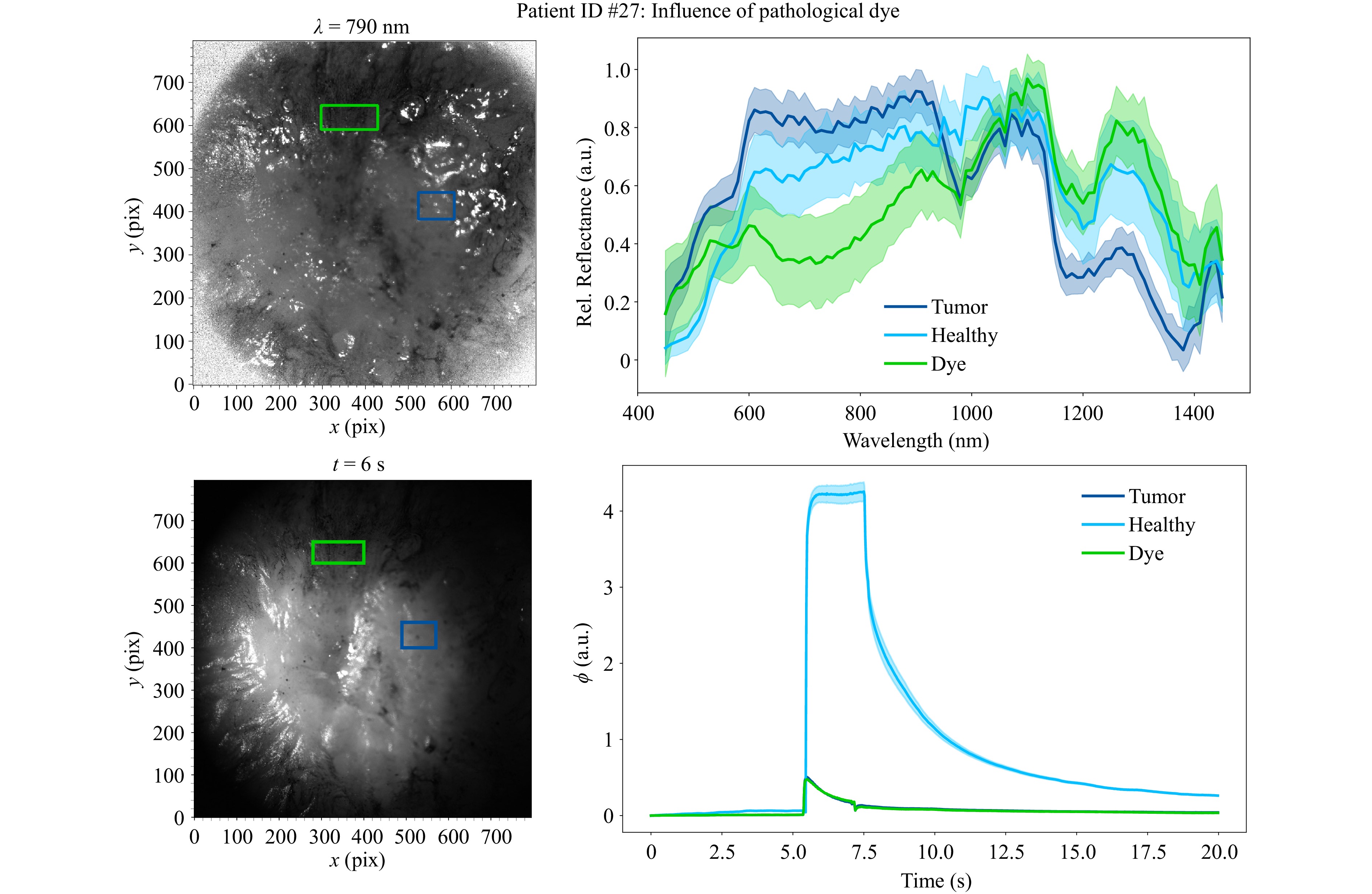
Fig. 12  Influence of pathological dye to HSI and FTP measurements. Left: Spectral and fringe images of tissue surface. The ROI for the tumor spectrum is marked in dark blue, the ROI of the dye contaminated tissue is marked in green. The ROI of the healthy tissue is not marked, because it is measured at another measurement position. Right: Spectral responses and indentation depths of the three different tissue types (tumor, healthy and dyed).

It is also evident that the HSI sensor has the advantage over the elastographic FTP in differentiating tumor boundaries, as can be seen in Fig. 6 and highlighted in Fig. 7. Furthermore, the HSI can also differentiate tissue across patients, as evidenced by the characteristic mean spectra in Fig. 5, unlike in the elastographic FTP, which measures different indentation depths for different patients, even for the same tissue types (see Fig. 10). The elastographic FTP principle also has its limits regarding sample thickness. Examining lamellas, which are too thinly sliced might yield false stiffnesses by the materials underneath, slightly move the tissue laterally due to the oblique force direction, or cause the surface of the tissue to also oscillate during indentation. The HSI can compensate for these cases as it is a stationary measurement.

It can thus be deduced, that a combination of the two presented modalities is a promising opportunity for robust bimodal tissue differentiation. Each modality benefits from the other, when used combined instead of independently, which is why the overall result can be improved by the mutual plausibility check.

Since a miniaturized version of this multimodal sensor system is intended for intraoperative use in the future, it is important to note that the difficulties identified here are only macroscopic impairments that may differ from an intraoperative use case. However, it can be assumed that even in this scenario, both sensor principles benefit from multimodal use. For pathological use, e.g. to embed areas of interest, the improvement through the multimodal combination has already been demonstrated within this work.

The presented results show a promising approach for tissue differentiation after breast surgery or subsequent pathological diagnostics. It has been shown that suspicious areas of the tissue’s surface can be identified by the HSI and checked for plausibility using elastographic FTP. The combination of both individual modalities allows for a much more reliable differentiation of tissue types than a single sensor. Furthermore, the independent measurement concepts can complement and validate each other. The combination of both modalities can help if one of the sensors is limited by its properties, e.g. due to contamination of the tissue surface with pathological staining agents.

In our study, we observed several aspects that should be considered in future studies. In one case for instance, the tissue surface showed remnants of pathological dyes that had been used in a necessary pathological preparation step as this is routinely used to mark margins. Attempts were made to clean it, but the dye had already soaked into the first cell layers. This affects the spectral analysis of the HSI sensor as shown above. Additionally ICG is often used for location of the tumor during surgical resection. ICG is excited between $ \lambda $ = 750 – 800 nm and the maximum fluorescence signal is detected around $ \lambda $ = 832 nm⁵⁷. According to the usage of ICG in some of the measured tissues, the corresponding spectral range is not used for evaluation. Furthermore, there is only a smaller difference in relative reflectance between the two tissue classes in the ICG spectral range compared to the spectral ranges emphasized in Fig. 4 (see also Fig. 5). It can therefore be assumed that the ICG spectral range is less meaningful for tissue differentiation compared to the highlighted spectral ranges.

Another aspect is the thickness of the tissue sample, which affects both HSI and elastographic measurements. In HSI measurements, the sample thickness influences the results due to the different penetration depth of the illumination light and thus the spectral response of the different tissue depths. The influence of the sample plate increases with decreasing tissue thickness. However, the signal strength to be expected from deeper layers is also low, so that the main signal should continue to emanate from the tissue surface. The thickness therefore plays a subordinate role for the HSI measurements. In contrast, for the elastographic measurements, the sample should have a certain thickness to minimize the influence of the materials underneath. The necessary sample thickness for indentation measurements depends for example on the applied force during measurements and the stiffness of the sample itself. It should be thick enough to support the indentation depth without any heterogeneities or different underlying materials. Although not further investigated in this study because the method used here does not correspond to any of the known standard macroindentation tests for hardness⁵⁸, the literature suggests that an indentation depth of about 10% of the sample thickness or even more should be sufficient for different tissue types and biomaterials^59–63. This value needs to be experimentally validated for this kind of macroindentation. The necessary sample thickness for indentation measurements with this setup, however, depends on a plethora of variables, for example:

1. The relative position between the cystocopic needle and the sample.

a. The distance between the cystoscopic needle and the sample influences both, the force acting on the sample and the area of indentation. As the distance increases, the air jet diverges, which decreases the pressure acting on the sample but also enlarges the indentation area. Hence, either the air pressure at the back of the cystoscopic needle must be increased dynamically as the distance to the tissue increases or the distance needs to be adjusted at a constant air pressure, both to keep the indentation force constant.

b. Different angles of inclination of the air jet impulse to the surface normal of the tissue change the indentation depth at each point of the tissue and the shape of the indentation volume overall, especially with complex topographies.

2. The elastic properties of the tissues samples: The indentation force and thus the applied air pressure must be able to sufficiently indent healthy tissue which might be stiffer in nature than other tissue types to have a baseline for comparison.

3. In an ex-vivo examination context, the weight of the tissue must be sufficiently high. Tissue samples that are too thin and therefore too light can be blown away by the air flow, if the air pressure is set too high.

4. The phase, which translates to the indentation depth in mm, may contain jumps of 2π depending on the reconstructed and unwrapped phase, especially for low visibility of fringes, which would influence the reconstructed indentation depth. Thus, the image processing algorithm used also has an influence on the reconstructed indentation depth.

Future research should conduct a model-based study using numerical methods such as the finite element method and verify the results with experimental measurements to better predict the indentation behavior.

Finally, the obtained spectral results show good comparability to other results in the literature, such as the spectra of healthy and malignant breast tissue presented by Kho et al.¹⁹. Prospective further measurements have to substantiate these initial results. In addition, further measurements of different special histological types of breast cancer or precursor lesions should be carried out with both sensors so that a differentiation between precursor lesion, invasive carcinoma, and connective tissue becomes possible.

Although currently being a laboratory setup, miniaturization of the sensor concept is a conceivable option to enable intraoperative use in MIS, since both sensor concepts are technically miniaturizable. The technical implementation will be particularly challenging in terms of real-time capability, as the evaluation for both sensor concepts is computationally intensive. Furthermore, the robustness of the measurement with regards to the medical application in MIS must be taken into account, as even the smallest movements lead to a different object view and the image acquisition must therefore also take place in a suitably short time to ensure high image quality. A possible option would be to integrate the FTP setup into a commercial endoscopic system as was shown by Aslani et al.^39–41. In the case of HSI, there also exist endoscopic implementations, such as shown in Köhler et al.²⁰ and Wirkert⁶⁴. All of the mentioned systems allow for a seamless combination of both subsystem to an overall bimodal endoscopic system.

The work described in this paper was conducted in the framework of the Graduate School 2543/2 "Intraoperative Multi-Sensory Tissue Differentiation in Oncology" (Project ID 40947457, subprojects A1, A2, C2, and C3) funded by the German Research Foundation (DFG - Deutsche Forschungsgemeinschaft). The authors thank Wala Hasnaoui and Sarra Dahene for their assistance in redesigning the electronics and fiber holders to improve the elastographic measurement system.