Simulation and experimental investigation of homogeneity measurement in side-polished transparent cylindrical materials

The refractive index homogeneity of optical materials is a critical parameter governing optical performance and is essential for applications in laser systems, high-resolution imaging, and precision optical manufacturing¹. In recent years, specialized cylindrical components, such as side-polished cylindrical transparent materials, have seen increasing use in laser diode beam shaping, fiber coupling, and deep-ultraviolet picosecond pulse laser resonators². At the same time, conventional cylindrical lenses and medical endoscope windows remain vital in applications such as LiDAR collimation and medical imaging^3–5. In all these applications, homogeneity directly determines system performance.

Optically, homogeneity refers to the spatial uniformity of the refractive index within a material. When a plane or cylindrical wave propagates through an inhomogeneous medium, localized refractive index variations introduce irregular wavefront distortions in the form of optical path differences. These distortions can increase beam divergence, elevate optical aberrations, and ultimately degrade system resolution and stability⁶.

Despite its significance, most established homogeneity measurement techniques—including the four-step phase-shifting method and wavelength-tuning interferometry^7–10—are designed primarily for planar optics. Their adaptation to side-polished cylindrical transparent materials is often hindered by geometric and surface characteristics, limiting accurate assessment, mainly due to two inherent technical issues:

1. First, the alignment of nonplanar Fizeau setups demands stringent confocal positioning of the transmission cylinder (TC), sample cylinder, and return cylinder with consistent angular relationships—a requirement that exceeds traditional planar assembly constraints, where minor three-dimensional (3D) assembly errors (radial offset, axial rotation, and curvature center offset) are amplified by cylindrical curvature and cannot be compensated for by planar error-correction models.

2. Second, in the cylindrical confocal interference system, taking transmission measurements as an example (consistent with back-surface interference), the surface figure errors of the return cylinder exhibit an R(−x, y) coordinate mirror-reversal characteristic. This characteristic is incompatible with the error-separation algorithms of conventional planar measurement methods, which are based on positive planar coordinate mapping, leading to distorted calculation results and the inability to effectively separate material homogeneity errors from coupled optical path differences.

Therefore, developing tailored measurement approaches for such components has considerable theoretical and practical value. To address this gap, this study systematically investigates a four-step phase-shifting interferometry method adapted for evaluating the homogeneity of side-polished cylindrical transparent materials. Combining theoretical analysis with simulation, the robustness of the proposed approach is further validated through experimental verification.

The Fizeau interferometer is one of the most commonly used configurations in interferometric measurement¹¹. Owing to its common-path design, it exhibits strong resistance to environmental disturbances and is therefore widely used in commercial interferometer systems. The four-step absolute measurement method is a mainstream technique for measuring optical homogeneity using Fizeau interferometers^12,13. Through dedicated algorithms and standardized measurement procedures, this method can effectively separate and eliminate the influence of surface figure errors from the transmission reference surface and other reference optical components on measurement results.

Building on the four-step measurement method for planar homogeneity, this study proposes a four-step homogeneity measurement method suitable for transparent cylindrical components. As shown in Fig. 1, the method follows the core measurement procedure, requiring sequential measurements of the empty cavity, transmission, front surface, and back surface. To accommodate the geometric characteristics of cylindrical components, the transmission cylinder (TC), transparent cylindrical sample, and cylindrical reflector must be precisely aligned in a confocal configuration. The specific measurement steps are as follows.

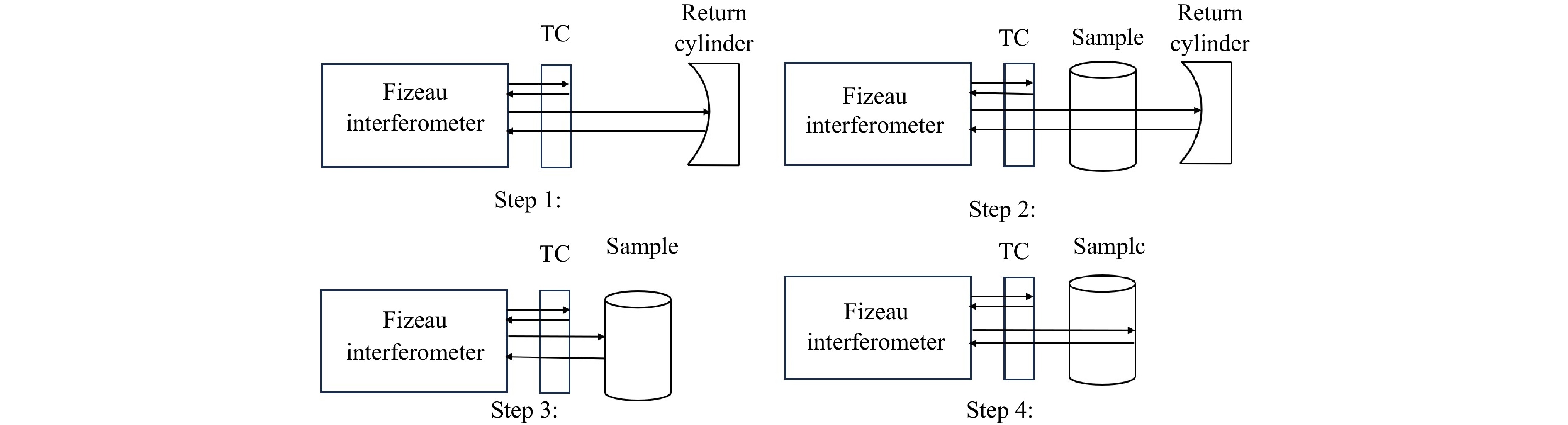
Fig. 1  Four-Step homogeneity measurement method for cylindrical surfaces.

A cylindrical coordinate system is established with the confocal position as the origin: the z-axis coincides with the optical axis, the x-axis corresponds to the radial direction of the cylinder, and the y-axis aligns with its generatrix. As shown in Fig. 2b, under confocal alignment, the three components maintain the same angular relationship θ. Consequently, once the TC aperture and radius of curvature are specified—together with the diameter of the side-polished transparent cylinder—and provided that the return cylinder aperture is sufficient to reflect all incident light, the interference region on the transparent cylindrical sample is uniquely determined, as shown by the green region in Fig. 2b.

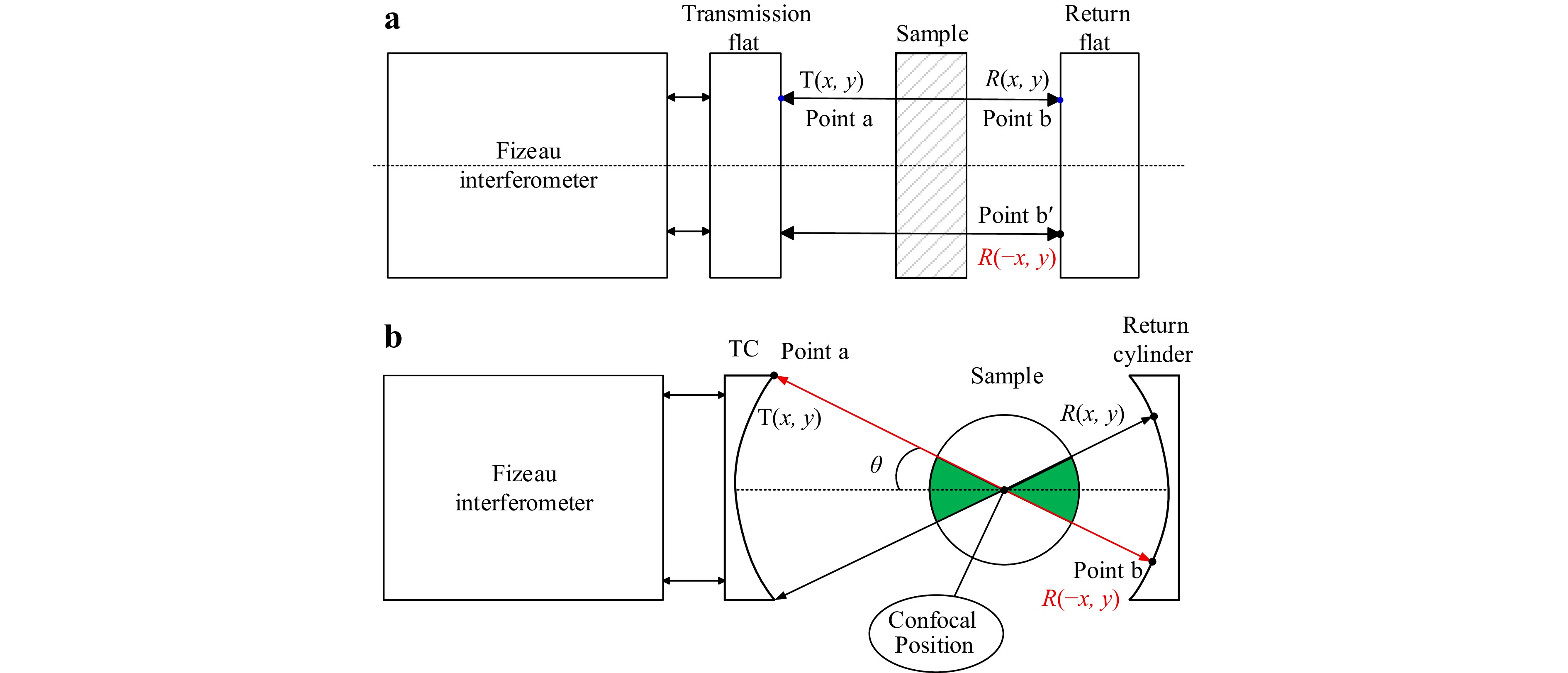
Fig. 2  Top view of confocal interference (XOZ plane).

First, the geometric positional relationship is analyzed. In the homogeneity measurement system for planar samples, the sample can be freely translated within a certain range, and its spatial position variation does not substantially affect the homogeneity measurement results. In contrast, the homogeneity measurement of transparent cylindrical samples must be strictly performed at the confocal position; therefore, the coordinate origin is set at the confocal point.

Second, the transmission mode for homogeneity measurement is considered. As shown in Fig. 2a, in the planar case, the light ray emerging from point a carries the reference mirror error T(x, y), and the corresponding point b on the reflection mirror carries the error R(x, y). In the cylindrical homogeneity measurement optical path, as shown in Fig. 2b, the red detection beam emitted from point a carries the reference mirror surface figure error T(x, y). After refraction and focusing, the beam reaches point b on the reflection mirror, where the corresponding surface figure error becomes R(−x, y) instead of R(x, y) as in planar measurements. Similarly, the surface figure error at the corresponding position on the back surface of the cylinder exhibits the same coordinate mirror-reversal characteristic. In MATLAB numerical modeling, this physical property of coordinate mapping reversal must be accurately incorporated into each step of the interference phase calculation to ensure the accuracy of the modeling results.

Step 1: The cylindrical reference beam is measured in the empty-cavity configuration. By adjusting the TC and return cylinder to the confocal position, the wavefront information W₁ under the empty-cavity condition is obtained through the following calculation:

T: surface figure error of the TC; R: surface figure error of the return cylinder.

Step 2: The side-polished transparent cylindrical sample is inserted and adjusted such that the TC, transparent cylindrical sample, and return cylinder are in the confocal position. At this stage, the reference beam propagates through the sample and interferes with the light reflected from the return cylinder. The wavefront information W₂ of the transmitted wavefront is obtained through interferometric calculation and contains the homogeneity information of the sample:

n: optical homogeneity variation; n₀: average refractive index of the material; F: surface figure error of the front surface; B: surface figure error of the back surface; t: thickness of the sample (for a cylindrical transparent sample, t equals the diameter D).

Step 3: The reference beam interferes with the light reflected from the sample front surface, yielding wavefront information W₃ that contains information about the TC and the front-surface figure of the measured sample:

Step 4: The reference beam interferes with the light reflected from the sample back surface, and wavefront W₄ is obtained, which carries information about the TC and the front-surface and back-surface figures of the measured sample:

Following the acquisition of wavefront information from the four steps described above, the refractive index distribution of the sample is reconstructed using a dedicated computational algorithm:

By determining the maximum difference in the refractive index distribution, the homogeneity value of the sample is derived:

In the simulation, three cylindrical models are initially constructed. The TC has an aperture of 60 mm and a radius of curvature of 150 mm; the return cylinder has an aperture of 50 mm and a radius of curvature of −50 mm; the side-polished transparent cylindrical sample has a diameter of 40 mm and a refractive index n₀ = 1.45702. The z-axis is designated as the optical axis, the x-axis as the radial direction, and the y-axis (y ∈ [−30, 30]) as the generatrix direction, with the three components coaxially aligned at the confocal position. The coordinate origin is defined at the geometric center of the sample, as illustrated in Fig. 3.

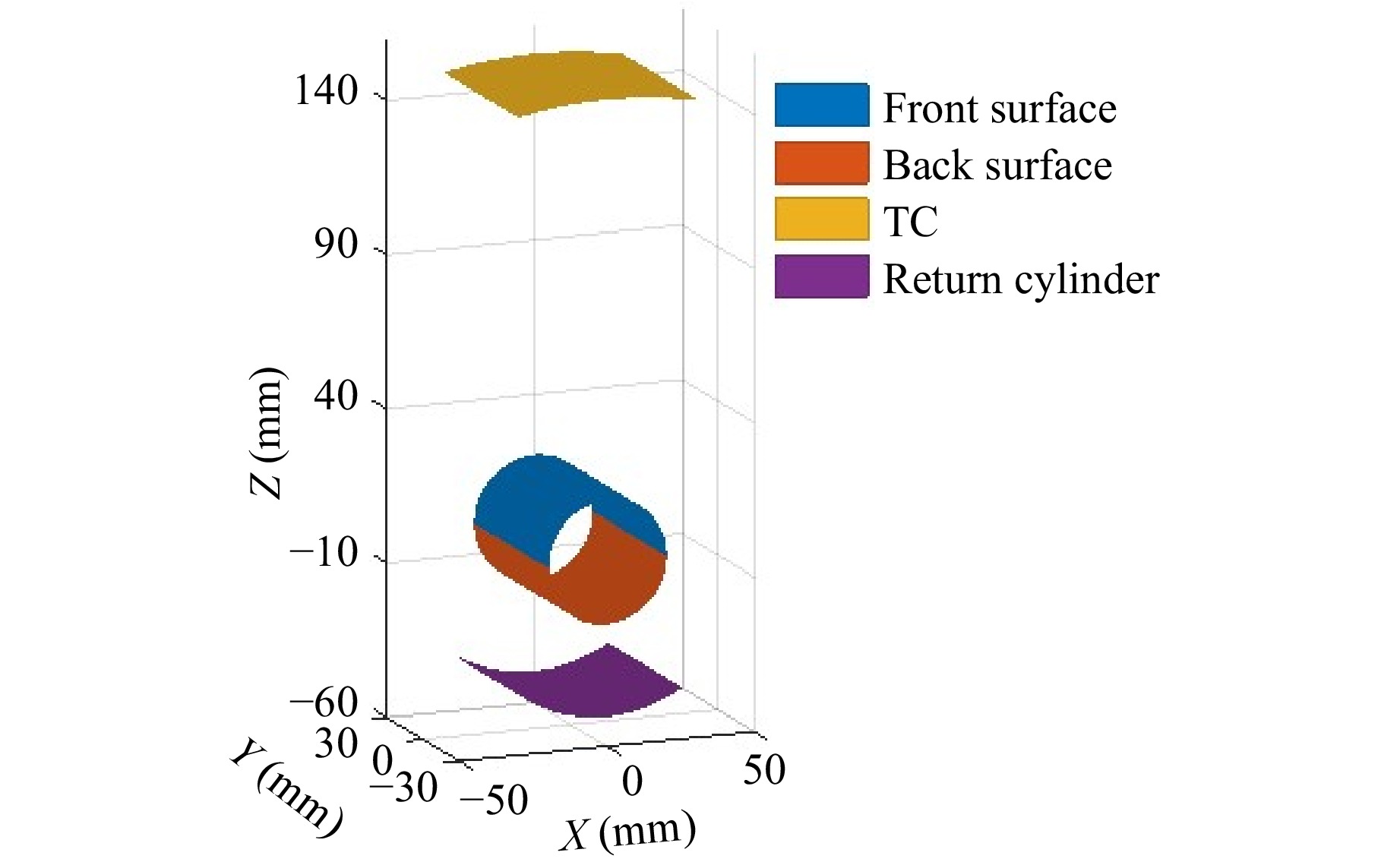
Fig. 3  Three-dimensional position plot in MATLAB.

As shown above, the aperture of the TC spans from −30 mm to 30 mm along the x-axis. Based on calculations of the identical included angle θ (Fig. 2), when the TC operates in full-aperture interference mode, the regions of the front and back surfaces of the transparent cylindrical sample involved in interference are confined to the x-coordinate range of −4 mm to 4 mm, while the interference region of the return cylinder spans −10 mm to 10 mm along the x-axis. Based on these calculated parameters, the required surface profiles are generated, as illustrated in Fig. 4.

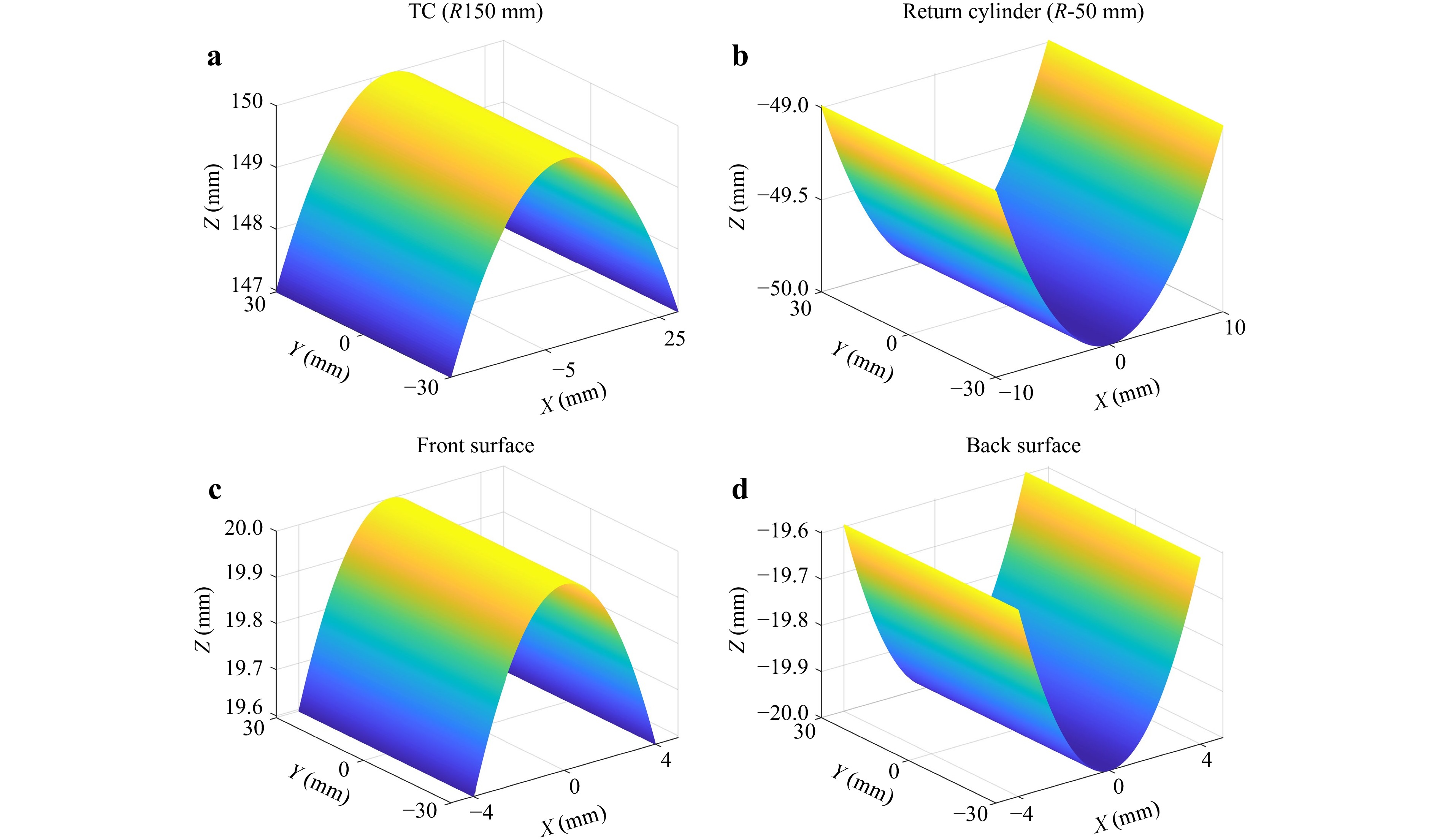
Fig. 4  Calculated interference-involved surface region.

In numerical simulations, relying solely on basic modeling approaches is insufficient. Given that the TC generally exhibits high surface figure accuracy, only a linear error along the y-axis is introduced in the simulation. This simplification effectively captures the tilt deviation typically encountered during TC alignment, as illustrated in Fig. 5.

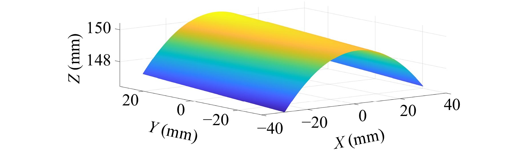
Fig. 5  TC surface profile with surface errors.

The linear error formula of the TC is given as follows:

Correspondingly, surface errors were also incorporated into the model of the return cylinder. In addition to tilt errors resulting from alignment, a saddle-type surface error was introduced to simulate rotational deviations and other asymmetries of the reflector about the optical axis encountered in actual measurements. To better approximate real experimental conditions, the amplitude of the saddle error in this study was intentionally set to a relatively high value, which also facilitated the clear identification of interference fringes. In the simulation, the surface of the return cylinder was therefore modeled by combining the saddle-shaped error described by Eq. 8 with the linear error given in Eq. 7; the resulting surface profile is illustrated in Fig. 6.

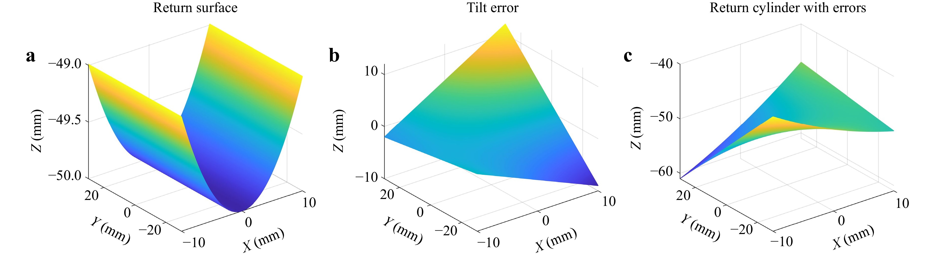
Fig. 6  Return cylinder with surface errors.

In addition to the saddle and linear errors described above, this study further introduced distinct forms of random errors on the front and back surfaces of the sample (Figs. 7 and 8) to better reflect the characteristics of actual machining and polishing processes. For the effective interference region on the front surface (Fig. 6c), a Gaussian random error field was constructed through the following steps. First, the target root-mean-square (RMS) error was set to λ and the peak-to-valley (PV) error to 8λ, where λ = 632.8 nm. After generating an initial Gaussian random noise distribution, a Gaussian filter with a standard deviation of 10 pixels was applied to restore the spatial continuity of the error. The amplitude was then scaled: the RMS error was first normalized to λ, followed by scaling to the target PV of 8λ, with simultaneous secondary calibration of the RMS. This procedure yielded a Gaussian random surface-profile error that met the required accuracy specifications for the front surface.

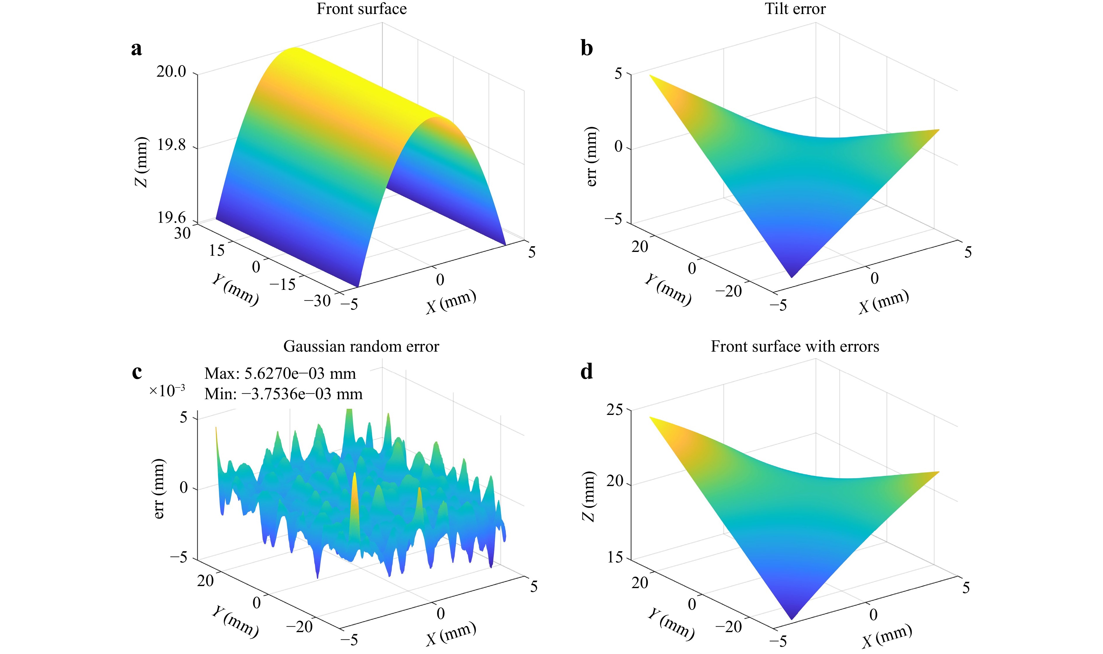
Fig. 7  Front surface of the transparent cylinder with introduced errors.

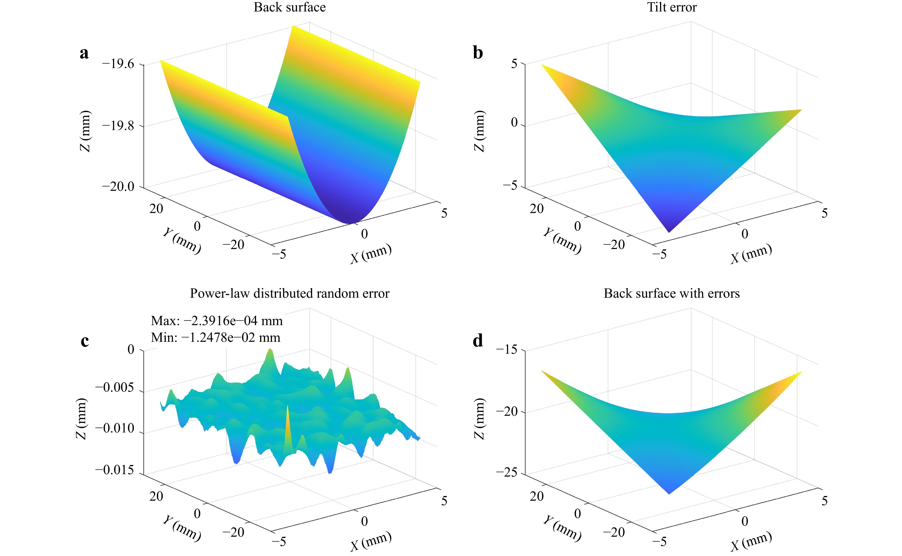
Fig. 8  Back surface of the transparent cylinder with introduced errors.

Unlike Gaussian short-range random errors, power-law distributed errors were introduced on the back surface of the sample to reproduce the multiscale characteristics of machining errors of the transparent cylinder, as shown in Fig. 8. These errors were used to simulate long-range correlated errors with fractal characteristics. The detailed procedure was as follows. First, the RMS error was set to 0.8λ and the PV error to 4.2λ. Uniform random numbers within the range of 0–1 were generated based on the effective interference area. After a power-law transformation (α = 1.5, where a smaller exponent indicates a rougher error), the random numbers were centered within the range of −0.5 to 0.5 to obtain the initial noise field. Gaussian filtering with a standard deviation of 15 pixels was then applied (different from the 10-pixel filtering parameter used for Gaussian errors) to match the characteristics of long-range errors. Subsequently, the RMS error was calibrated to 0.8λ and then scaled to the target PV value of 4.2λ, with simultaneous secondary calibration of the RMS error. Ultimately, a power-law distributed long-range correlated error distribution that met the precision requirements was obtained.

Under ideal conditions, when the material of an optical element is specified, its refractive index at a given wavelength is a fixed constant. However, during the actual manufacturing process, the refractive index distribution within the material is not perfectly homogeneous. To achieve accurate simulation of the homogeneity detection system, refractive index inhomogeneity was introduced into the simulation model. In the MATLAB simulation environment, the characteristics of gradient-index materials can be defined. This study adopted a radial gradient refractive index distribution within the XOZ plane, and the expression of this gradient refractive index is expressed as follows:

Here, n₀ denotes the refractive index at the center of the optical element, n_r2 is the radial quadratic refractive index coefficient, and r represents the radial distance from any point on the transparent cylindrical sample (XOZ plane) to the origin. In the simulation, the transparent cylinder has a radius of 20 mm. It is known that n₀ = 1.45702 (632.8nm). Assuming the maximum difference in the internal refractive index of the element is Δn = 1 × 10⁻⁵ and setting n_r1 = 0, the parameters in Eq. 9 are determined as follows: and n_r2 = −2.5 × 10⁻⁸. The refractive index distribution curve of fused silica within the radial aperture range of the cylinder (at z = 0) is shown in Fig. 9a. The result obtained by evaluating Eq. 9 is as follows:

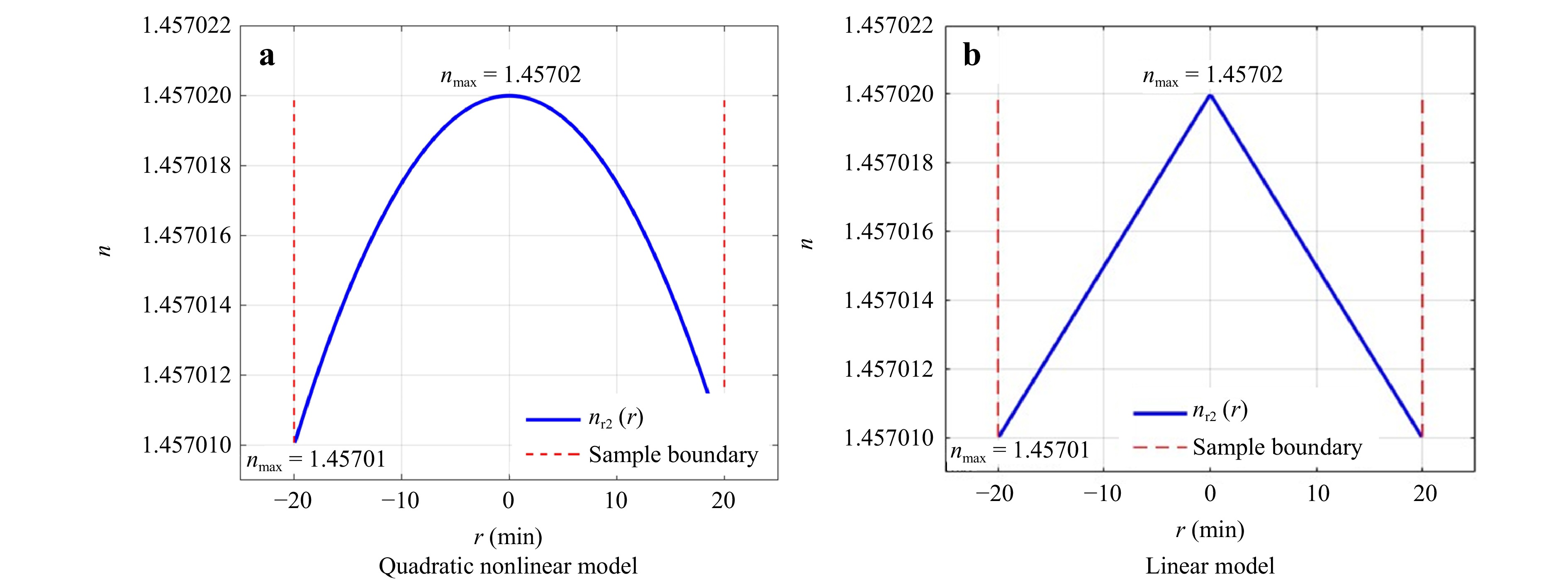
Fig. 9  Radial refractive index variation (XOZ, z = 0).

The quadratic nonlinear model not only better aligns with actual preparation processes at the physical implementation level but also demonstrates significant advantages in aberration correction in terms of optical performance. In contrast, the linear model can only roughly describe the refractive index distribution under very limited approximation conditions. As shown in Fig. 9, when introducing a maximum homogeneity deviation on the order of 10⁻⁵, the refractive index distribution curve characterized by the quadratic nonlinear model also exhibits superior smoothness. Therefore, the quadratic nonlinear model was adopted to describe the refractive index variation in this study.

Following the construction of the simulation model, the four-step homogeneity detection method was employed to simulate the corresponding interferograms for empty-cavity interference, transmission interference, front-surface interference, and back-surface interference, as shown in Fig. 10. After phase unwrapping was applied to the extracted phase data, the resulting surface profiles obtained from phase-shifting interferometry are presented in Fig. 11.

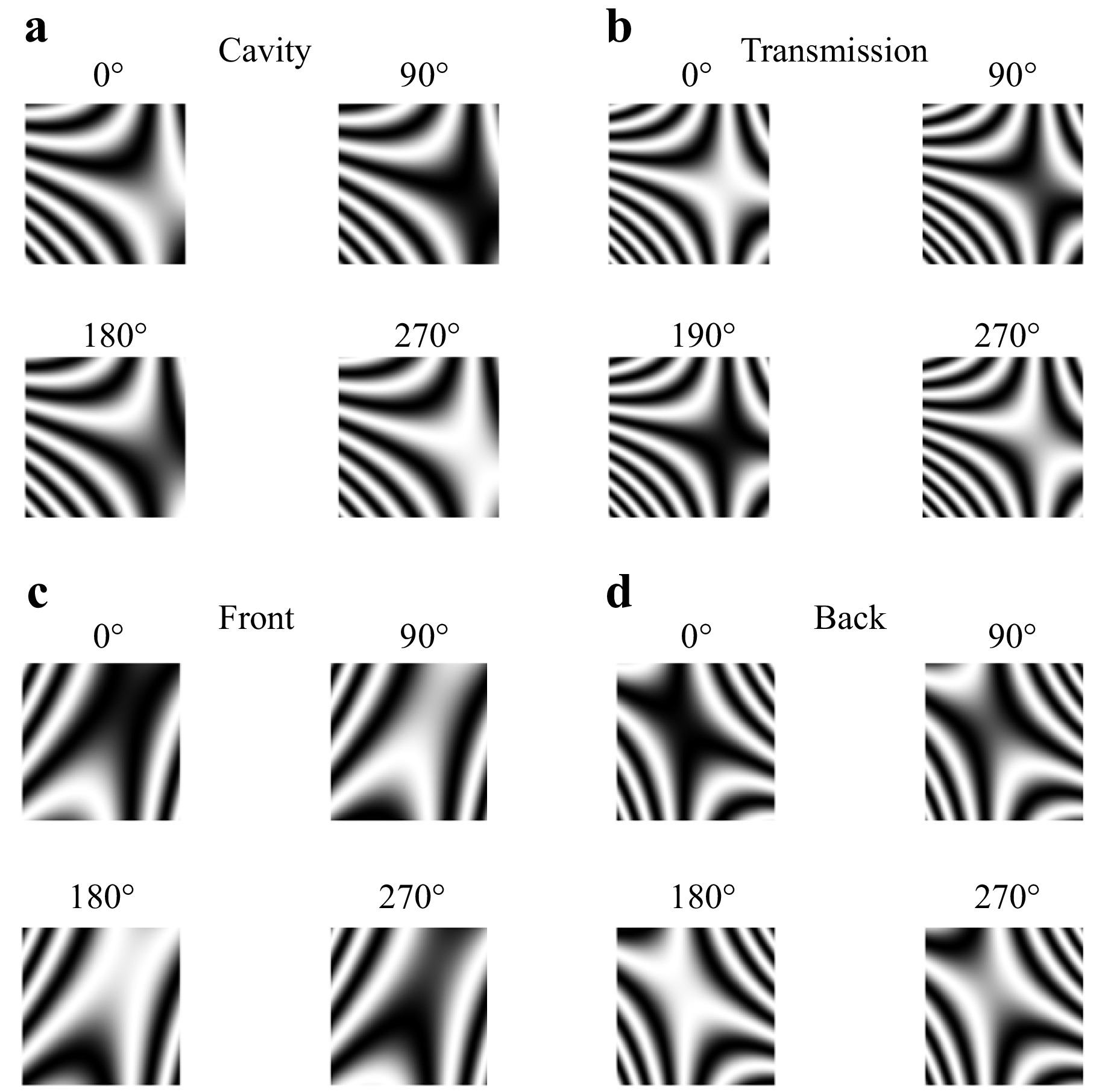
Fig. 10  Four-step phase-shifting interferograms.

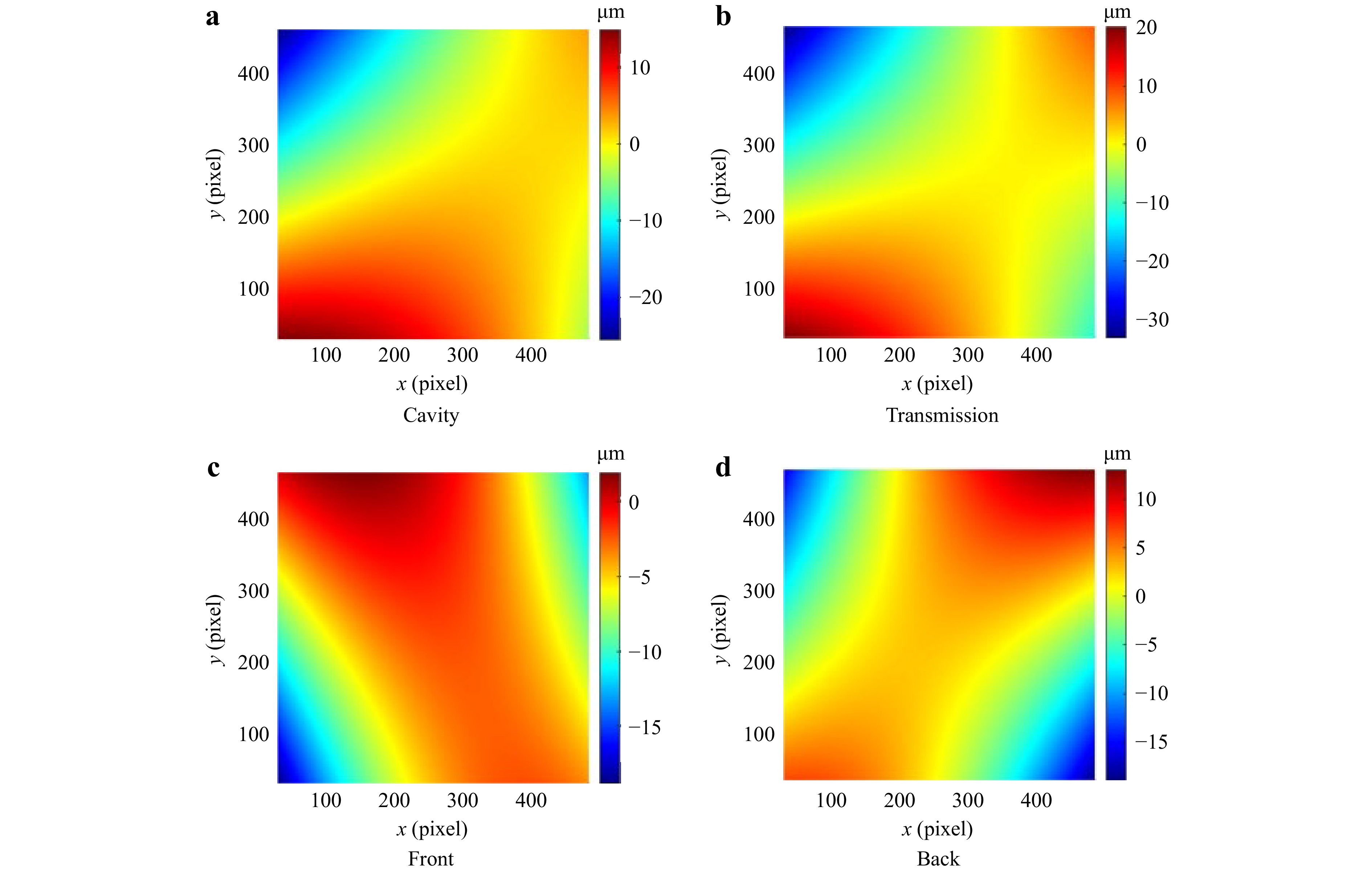
Fig. 11  Simulated phase-shifted interferometric surface profiles.

Based on the simulated phase-shifted surface profiles, the refractive index distribution of the transparent cylindrical sample was derived using Eq. 5. The results showed a calculated maximum refractive index difference of 9.9999 × 10⁻⁶. Compared with the preset maximum difference of 1 × 10⁻⁵ introduced in the simulation, the residual error was only 8.0319 × 10⁻¹¹, which is effectively negligible. This outcome confirms the feasibility of the four-step cylindrical homogeneity detection method proposed in this study. A detailed numerical comparison is presented in Fig. 12.

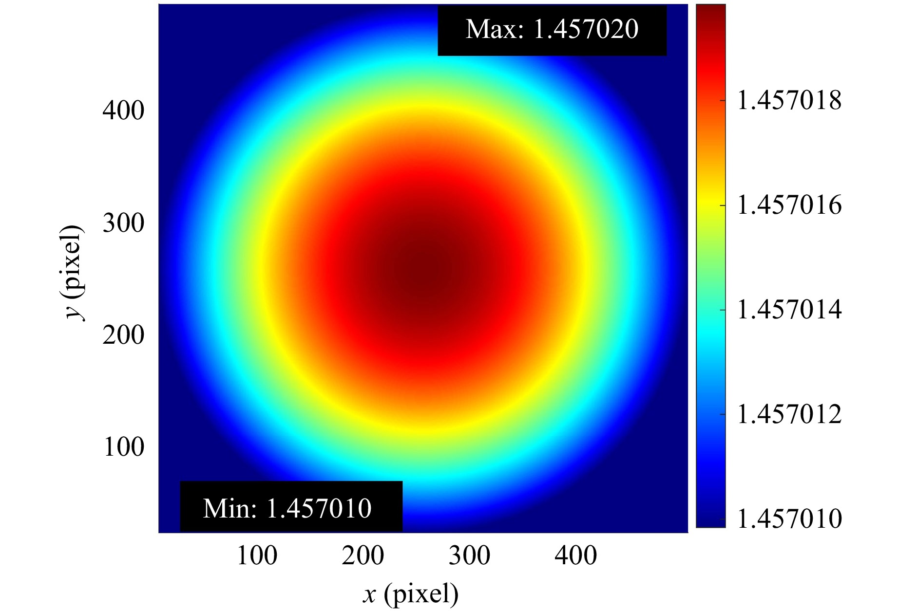
Fig. 12  Refractive index distribution.

For this experimental study, a 2-inch Fizeau interferometer manufactured by Suzhou H&L Instrument Co., Ltd. was used, with a 2-inch TC serving as the reference optic. The test sample was a side-polished transparent cylinder with a diameter of 41 mm, while a plano-concave cylindrical mirror was used as the return cylinder. This component is specifically designed to reflect all light emitted by the reference optic back along its original optical path. A schematic diagram of the experimental configuration is shown in Fig. 13.

Fig. 13  Experimental setup.

All alignment operations in this experiment followed the same precision standard. Fig. 14 shows the calibration result of the alignment accuracy used in the experiment, where each scale on the left side of the device represents 0.5 mm, and a 0.5 mm movement on the left scale corresponds to 50 grid movements on the right side. Based on this relationship, the alignment accuracy of the experiment was determined to be 0.01 mm.

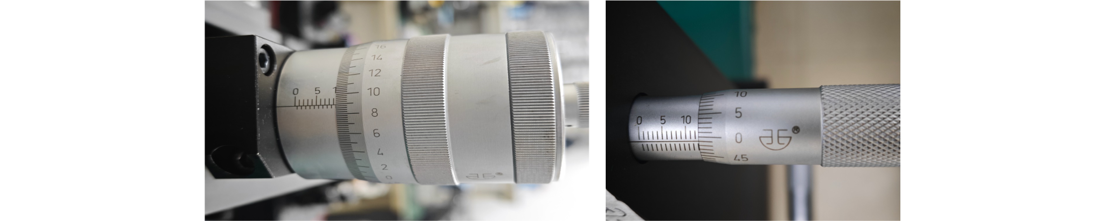
Fig. 14  Alignment accuracy.

The entire experimental setup was built on an air-floating vibration-isolation platform. For the temperature and humidity parameters during the experiment, contemporaneous environmental monitoring records from the laboratory were retrieved. Fig. 15 shows the temperature and humidity data recorded during the experiment, and Fig. 16 presents the airflow control device used in the experimental environment.

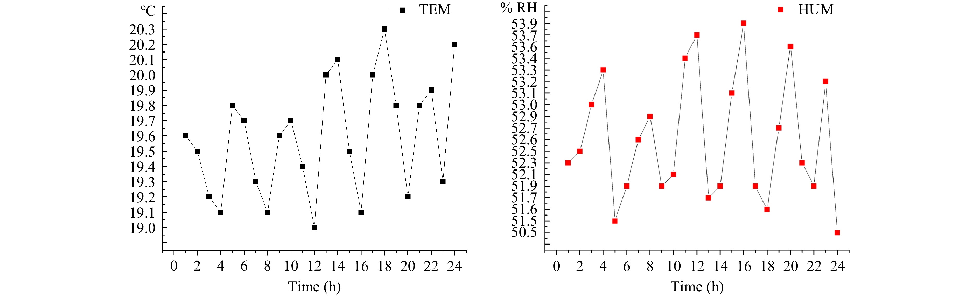
Fig. 15  Temperature and humidity monitoring curves.

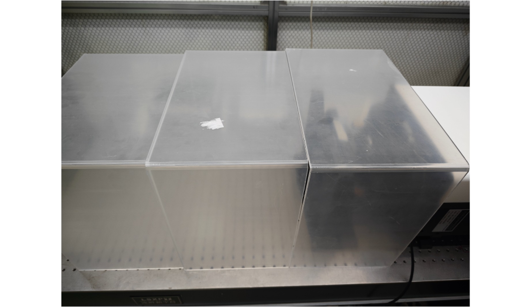
Fig. 16  Airflow control device.

Under conditions of 20 °C and standard atmospheric pressure, the experimental data corresponding to empty-cavity interference, transmission interference, front-surface interference, and back-surface interference were measured using the four-step cylindrical homogeneity detection method. The average values obtained from ten measurements are presented in Fig. 17. Empty-cavity interference: PV = 0.2252 μm, RMS = 0.0295 μm. Transmission interference: PV = 1.7512 μm, RMS = 0.2127 μm. Front-surface interference: PV = 2.2324 μm, RMS = 0.2808 μm. Back-surface interference: PV = 3.6334 μm, RMS = 0.4480 μm.

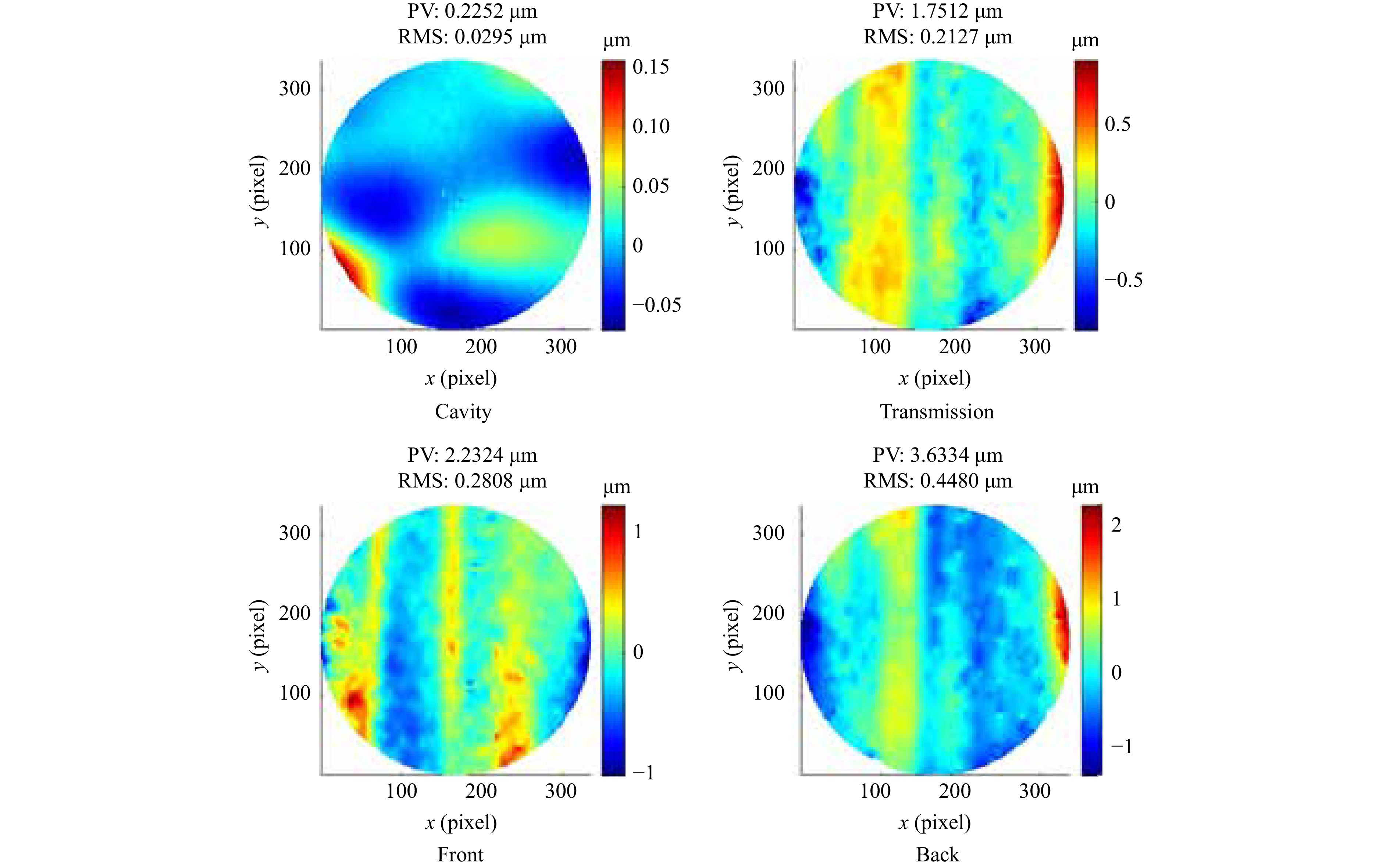
Fig. 17  Results of the first homogeneity measurement using the four-step method.

To confirm the reproducibility of the proposed detection method, the experiment was repeated at different time points under stable environmental conditions. The averaged results from these repeated trials, as shown in Fig. 18, demonstrate good consistency and validate the reliability of the measurement procedure. Empty-cavity interference: PV = 0.2251 μm, RMS = 0.0295 μm. Transmission interference: PV = 1.7331 μm, RMS = 0.2129 μm. Front-surface interference: PV = 2.2682 μm, RMS = 0.2812 μm. Back-surface interference: PV = 3.6317 μm, RMS = 0.4488 μm.

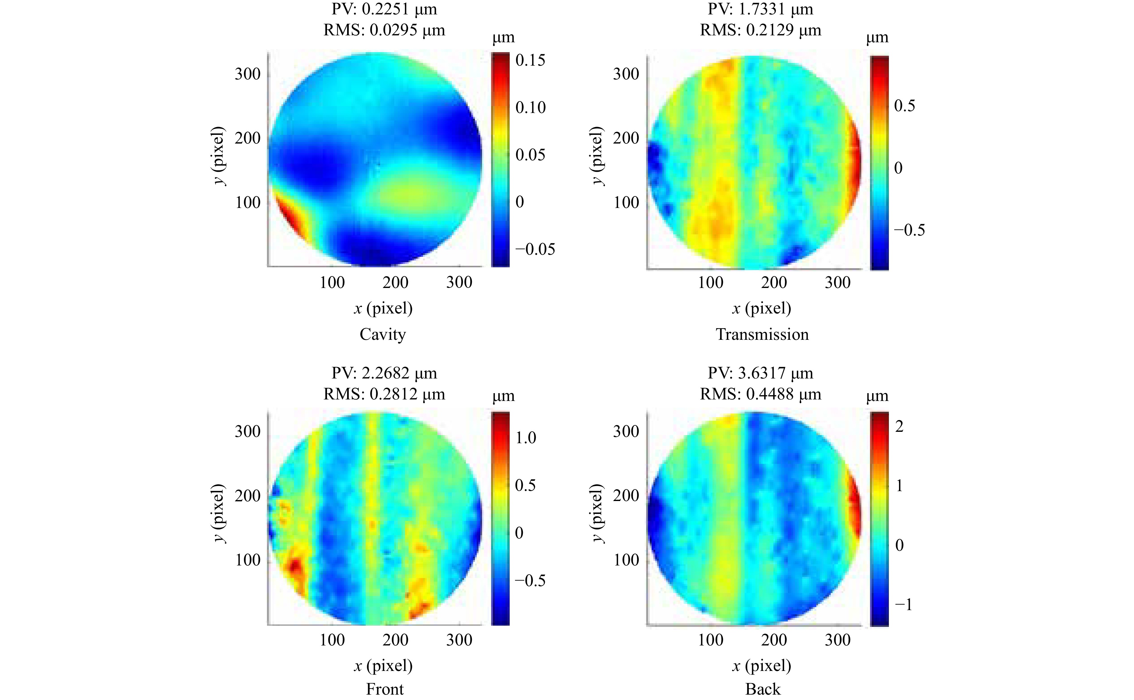
Fig. 18  Results of the second homogeneity measurement using the four-step method.

Based on the aforementioned experimental results, the refractive index distribution of the sample was calculated using Eq. 5. From Fig. 19a, the values of n(x, y)_max and n(x, y)_min are 5.0167 × 10⁻⁶ and −8.8745 × 10⁻⁶, respectively. The refractive index distribution obtained from the second measurement is presented in Fig. 19b, where the values of n(x, y)_max and n(x, y)_min are 4.5972 × 10⁻⁶ and −8.9357 × 10⁻⁶, respectively.

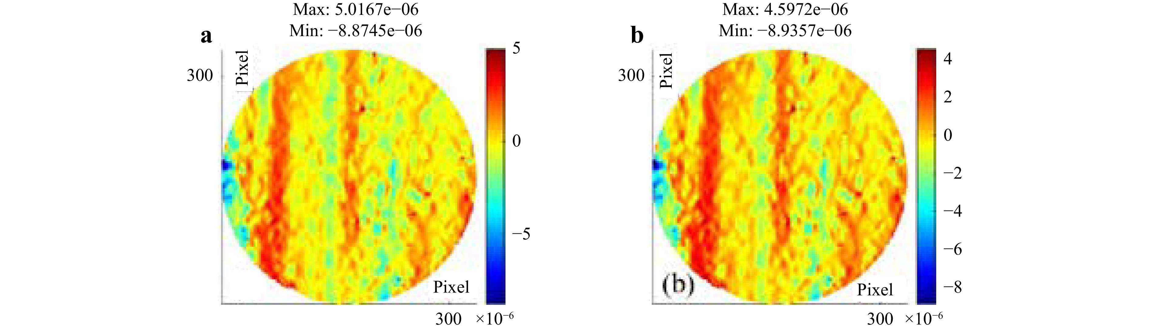
Fig. 19  Refractive index distribution. a first measurement; b second measurement.

Using Eq. 6, the two homogeneity measurement results were calculated as hom₁ = 9.5802 × 10⁻⁶ and hom₂ = 9.3331 × 10⁻⁶. The results are in good agreement, with a relative deviation of only 2.7%.

A measurement uncertainty analysis was performed for the four-step cylindrical homogeneity detection method proposed in this study. The measurement uncertainty of this method mainly includes system measurement repeatability, sample thickness calibration error, sample refractive index calibration error, off-axis rotation error, ambient temperature and humidity effects, and sample curvature inconsistency. This study focuses on system measurement repeatability, sample thickness calibration error, and sample refractive index calibration error.

Measurement uncertainty was derived from the repeatability results of each measurement step, and the calculation method is given by Eq. 11 as follows:

where ΔW₁ denotes the measurement repeatability of the cavity, ΔW₂ denotes the measurement repeatability of the sample transmission wavefront, ΔW₃ denotes the measurement repeatability of the sample front surface, and ΔW₄ denotes the measurement repeatability of the sample back surface. As shown in Fig. 20, twenty data points are presented: the first ten data points belong to the first measurement group, and the last ten data points belong to the second measurement group.

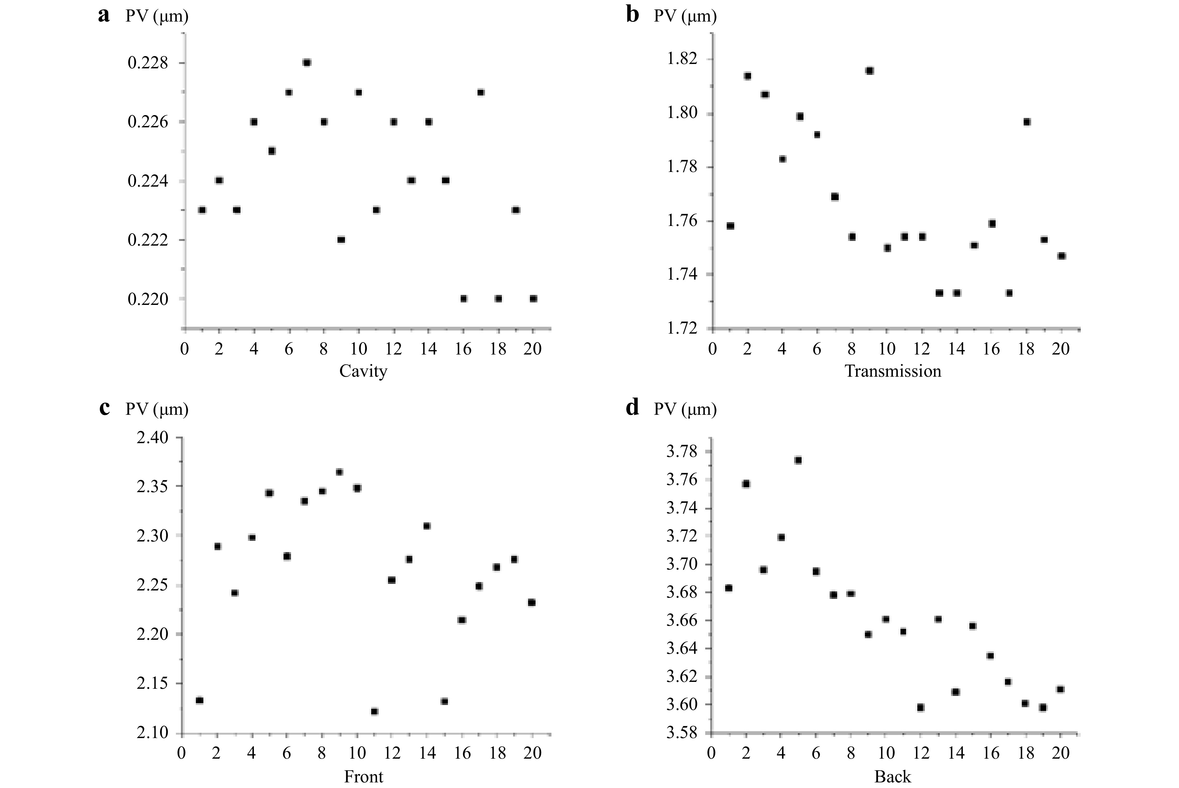
Fig. 20  Twenty measurement data points.

According to the measurement data obtained using the aforementioned four-step homogeneity detection method, the measurement repeatability is summarized in Table 1.

In this study, the entire measurement system was placed on an air-floating platform. The laboratory environment was controlled at 20 °C and one standard atmosphere. The calculated values of u₁ for the two groups are 1.0901 × 10⁻⁶ and 0.8646 × 10⁻⁶, respectively.

In the calculation of refractive index homogeneity, the result is inversely proportional to the measured sample thickness. The calculations were performed assuming a thickness measurement accuracy ΔD of 0.01 mm (10 μm). For a sample with thickness t (D = t mm), the measurement uncertainty introduced by the sample thickness calibration error was obtained by taking the partial derivative of parameter d using Eq. 5. The measurement uncertainty u₂ introduced by the thickness error Δt is given by:

When the measured result Δn(x, y) is 9.5802 × 10⁻⁶ or 9.3331 × 10⁻⁶, the corresponding values of u₂ are 2.3366 × 10⁻⁹ and 2.2764 × 10⁻⁹, respectively, which are much smaller than the measurement uncertainty introduced by measurement repeatability.

In the calculation of refractive index homogeneity, the result is directly proportional to the nominal value of the sample refractive index. In this study, the refractive index variation Δn of the sample was calculated with an error of 0.00001. The nominal refractive index of the material sample is n₀, and the measured value of n₀ in this study is 1.45702. The measurement uncertainty introduced by the refractive index error was obtained by taking the partial derivative of parameter n₀ using Eq. 5, and the resulting measurement uncertainty is denoted as u₃, expressed as follows:

When Δn is 0.00001, the calculated value of u₃ is 0.145 × 10⁻⁶.

The uncertainty components introduced above are independent and uncorrelated. According to the law of uncertainty propagation, the measurement uncertainty of the proposed four-step method for cylindrical homogeneity is expressed by Eq. 14, and the expanded uncertainty is expressed by Eq. 15:

The expanded uncertainty expression is given as

where k is the coverage factor. When k = 2, the confidence probability P = 95.45%. Therefore, the measurement uncertainty analysis results for cylindrical optical homogeneity obtained in this study are shown in Table 2 below.

In this study, only selected sources of measurement uncertainty for cylindrical homogeneity were quantitatively analyzed, and the influencing factors considered remain limited. In future work, the uncertainty evaluation framework will be further improved, and systematic analysis and experimental verification will be performed on additional potential error sources to enhance the reliability and accuracy of cylindrical homogeneity measurements.

A four-step absolute measurement method for quantitatively evaluating the refractive index homogeneity of side-polished cylindrical transparent optical elements using a Fizeau interferometer was established in this study, successfully addressing the technical challenge of quantitatively measuring refractive index homogeneity in such elements. By adopting a confocal coordinate system and a structured measurement sequence, this method reliably separates surface figure errors from material inhomogeneity. Simulation results confirmed the theoretical validity of the method. When a maximum refractive index difference of 1 × 10⁻⁵ was introduced, the retrieved value was 9.9999 × 10⁻⁶, with a negligible residual of 8.0319 × 10⁻¹¹. Experimental verification under stable conditions yielded two homogeneity measurements of 9.5802 × 10⁻⁶ and 9.3331 × 10⁻⁶. The relative deviation between them was 2.7%, demonstrating good repeatability. This deviation likely resulted from practical factors such as minor environmental fluctuations and sample repositioning errors, further confirming the robustness of the method under practical conditions. In addition, three sources of uncertainty were quantified in this study. The uncertainties of the two measurements were 1.0997 × 10⁻⁶ and 0.8767 × 10⁻⁶, respectively, and the corresponding expanded uncertainties were 2.1994 × 10⁻⁶ and 1.7534 × 10⁻⁶. Additional uncertainty sources will be quantified in future work to further improve measurement accuracy. In conclusion, this study provides an effective solution for the homogeneity measurement of side-polished cylindrical transparent optical elements, helping to address a gap in related measurement technologies.

This study was supported by the National Key R&D Program of China (Project No. 2022YFF0607701). The authors thank Jincheng Zhuang for technical support. The authors also thank Jianjun Hou and Genxing Jin for assistance with the experimental setup.