Contributions of holography to the advancement of interferometric measurements of surface topography

The historian Sean F. Johnston has observed that “…just as holography allows observers to see an image with multiple perspectives, exploring its history demands a range of viewpoints¹.” Holography has attracted microscopists, quality control engineers, scientists, and even artists. This paper views holography from the perspective of developers of optical interferometers for measuring surface topography.

Comparing holography with interferometry requires some impressions of how these two technologies differ, and how they are the same. Based on the works of Gabor² and Leith³, and consistent with widely-accepted definitions of the technique^{4, 5}, holography is a two-step process: (a) Recording the amplitude and phase of a propagating wavefront as an intensity image—the hologram—using interference with a reference wavefront, followed by (b) reconstruction of the propagating wavefront from the intensity image using optics or a digital simulation. Fig. 1 summarizes these two steps. The reconstruction of the propagating wavefront enables changing the image focus and perspective, leading to the famous three-dimensional (3D) imaging capabilities of the technique. One of the miracles of holography is that despite the sometimes-indecipherable holographic patterns, it is not only possible to create these 3D images, but also to quantitatively analyze vibrations, deformations and shape using multiple and time-averaged exposures⁶.

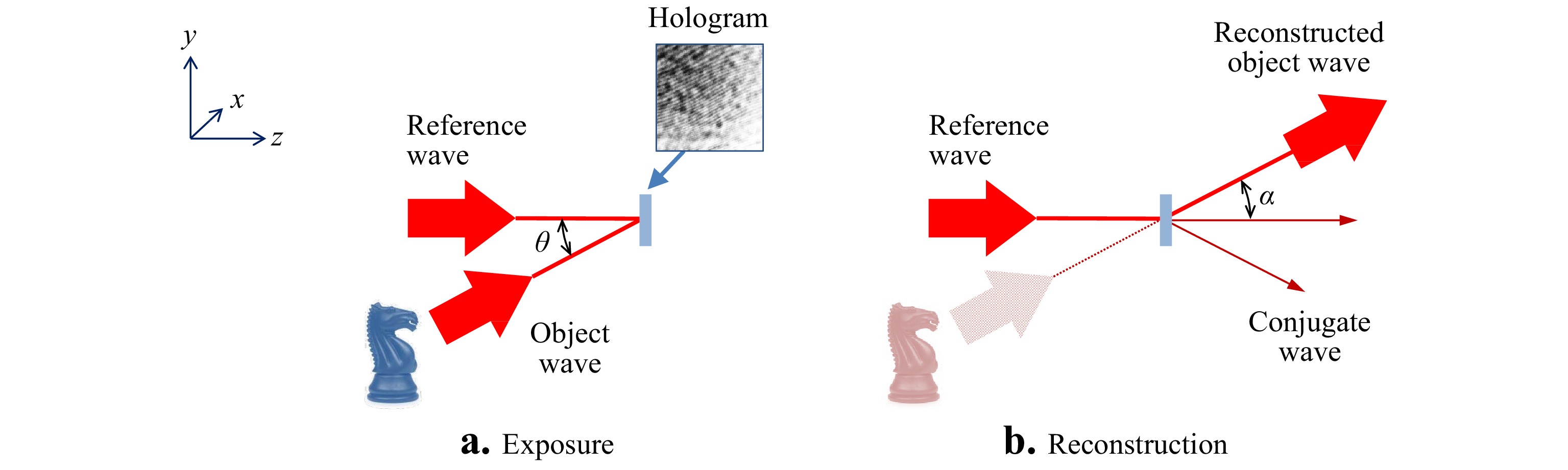
Fig. 1  a Creation of a hologram and b reconstruction of the propagating object wave by diffraction.

Interferometry is also a two-step process, but classical interferograms are created and interpreted in ways that are distinguishable from holography. Fig. 2a illustrates interferometry using two nearly flat optical parts illuminated from above with spectrally-filtered light. Fig. 2b shows a traditional conversion to surface topography, where the bright and dark fringes are interpreted as contour lines at increments approximately equal to half the illumination wavelength⁷. Interferometry does not normally include the uniquely “holographic” step of recreating a propagating wavefront from the recording of the original scattered light. For surface topography measurements, the interferogram is most often captured at the position of best focus of an imaging system, and the structure of the interference pattern is mapped directly to surface coordinates⁸.

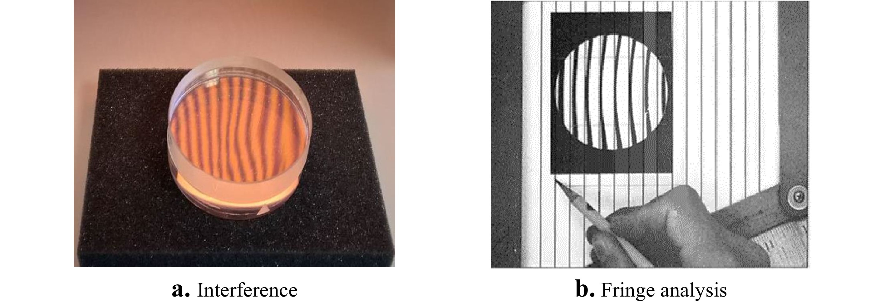
Fig. 2  a Formation of interference fringes and b manual analysis based on fringe straightness. The fringe analysis image is from a 1977 handbook on interferogram analysis, courtesy of Zygo Corporation.

Notwithstanding these distinctive characteristics, interferometry and holography share the common principle of holistically recording the magnitude and phase distribution of propagating light reflected from an object as an intensity pattern, using the interference of reference and object waves⁹. The availability in the 1990s of electronic cameras with sufficient sampling density to record holograms digitally reinforced this commonality, allowing for direct interpretation in magnitude and phase of complex holographic recordings. The physically unique step of holographic reconstruction of a propagating wavefront has become a software model, which can be applied equally well to holograms and to interferograms. This evolution has brought the two techniques even more closely together, and the convergence continues today.

The goal of this paper is to discover concepts and inventions in holography that have contributed to the advancement of classical interferometric methods that are not normally thought of as holography. We have chosen seven illustrative examples of such connections: phase shifting interferometry, carrier fringe interferometry, suppression of coherent noise, digital refocusing, computer generated holograms, measurements of rough surface topography, and 3D imaging theory. We do not attempt here to provide a comprehensive review of any one of these individual topics. Rather, our goal is to highlight some of the significant and perhaps surprising developments in interferometer design, data processing and physical optics theory inspired by holography.

The shared fundamental principle of capturing wavefront information in holography and interferometry is also a common difficulty, in that the complex amplitudes of the recorded light field are locked inside an intensity pattern. In modern interferometers for topography measurement, this problem is most often solved by phase shifting interferometry (PSI) or comparable heterodyning techniques¹⁰. Described most generally, the PSI idea is to record multiple interferograms that are nearly identical apart from a phase shift between them, so as to provide enough information to extract the object light phase and intensity. Although the history of PSI is usually traced to homodyne and heterodyne displacement measurements¹¹, it can be meaningfully argued that PSI for areal measurements came first to holography and then independently to interferometry.

To view the conceptual development of PSI from the perspective of holographic methods, it will be useful to write down the basic mathematical principles of holography. In the holographic exposure shown in Fig. 1a, we have at the hologram plane a light field reflected from an object defined by the complex representation

and a reference light field represented by

For the realization of Gabor in-line holograms, the recording tilt angle $ \theta $ shown in Fig. 1a is close to zero. The result after square-law detection is the interference pattern

which reduces to the familiar two-beam interference equation

In both holography and interferometry, what interests us is the phase $ {\phi _o} $ and intensity $ {I_o} $ of the original object wave, rather than this periodic cosine function. The problem is essentially the same for both technologies; however, the problem manifests itself differently in holography and interferometry.

In film-based holography, the exposed hologram is illuminated with the original reference to create the holographic image. By careful control of the photographic process, the amplitude transmissivity of the hologram can be made proportional to the intensity of the original interference pattern¹². The synthesis of the holographic image is represented mathematically by multiplying the intensity pattern of Eq. 3 by the complex amplitude of the reference wave:

In Eq. 5 it is only the final term containing $ {u_o} $ that is of interest. In the original in-line Gabor holograms, the reference $ {u_R} $ is a diverging wavefront, and the reconstruction includes overlapping, coaxial diffracted beams. The relative divergence is insufficient for separating the original wavefront $ {u_o} $ from the conjugate wavefront $ {u_o}^* $, resulting in a degradation of the desired image. This is where the phase shifting idea comes into play.

As Gabor and Goss describe in a 1966 retrospective of early developments, a holographic interference microscope constructed during the period 1951-56 isolates the desired wavefront using polarizing optics to introduce phase shifts between two otherwise identical holograms¹³. Gabor's quadrature microscope is shown in the simplified diagrams of Fig. 3. A key component is a special prism with a coating that introduces a quarter-wave phase shift, labeled ${\lambda \mathord{\left/ {\vphantom {\lambda 4}} \right. } 4}$ in Fig. 3a, between reflected and transmitted light. After exposure, we have two holograms with fringe patterns that we can write in simplified form as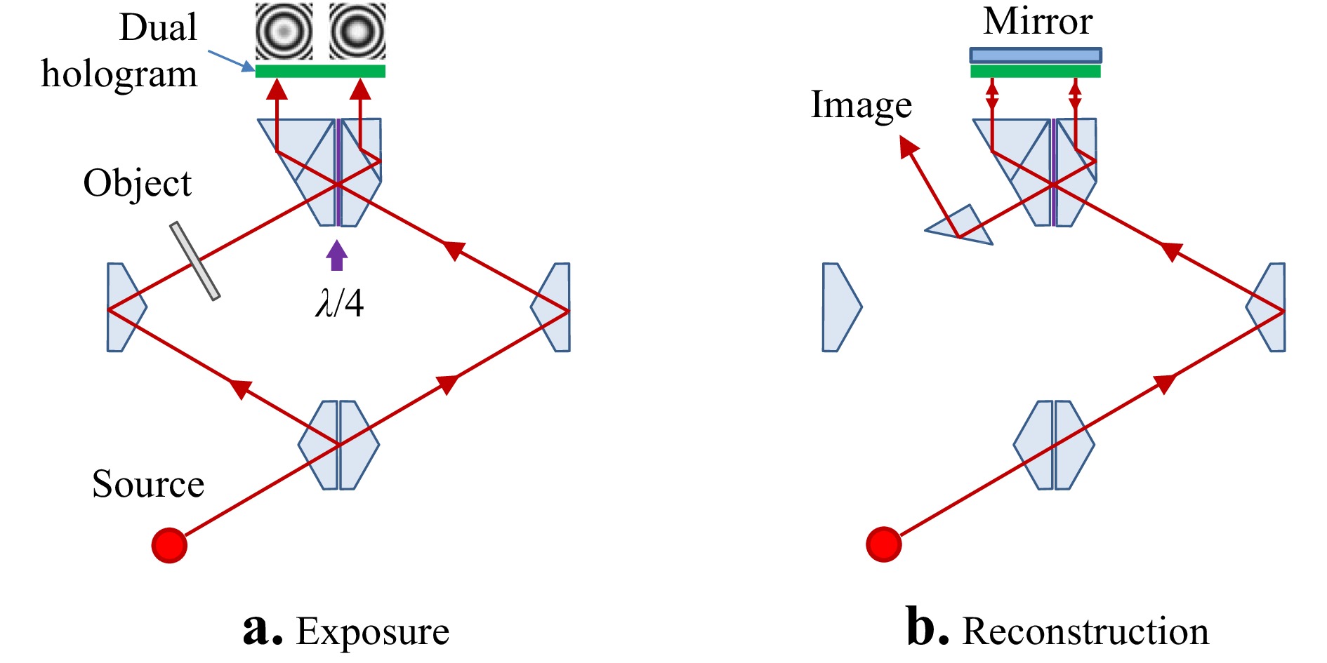

Fig. 3  Quadrature holography proposed by Gabor et al. in 1951. Lenses have been left out for simplicity in the diagram.

where constant terms have been set aside since these can be determined by other means. If we now illuminate with two copies of the reference wave that are also shifted in phase by a quarter wave as in Fig. 3b, the coherent sum of the reconstructed images is proportional to a net result

where again constant terms have been set aside. The reconstruction is recognized as a complex-valued amplitude, described as a “total wavefront reconstruction.”¹³ At the same time, the conjugate wavefronts generated by the two holograms cancel, at least in principle. In practice, additional elements are needed to precisely tune the phase shift and to adjust the intensities of the two reconstructed wavefronts to achieve this goal. One of the many remarkable features of this ingenious arrangement is that the calculations leading to Eq. 8 are performed entirely in optics, without electronic detection or digital data processing, in what can be reasonably described as an early all-optical computer of complex mathematical functions.

Although there have been modern implementations of optical quadrature holography¹⁴, the legacy of the apparatus of Fig. 3 is not so much its specialized design, as it is the concept of introducing phase shifts between otherwise identical interference intensity patterns to recover complete wavefront information. This basic idea was soon adopted for non-holographic interferometry. Interferograms, like holograms, are also created by mixing a reference wave with light that is reflected from the object. Most often it is assumed that there is a linear relationship between the phase $ {\phi _o} $ and the object surface height $ {h_o} $ as a function of surface coordinates $ x,y $, with a factor of two related to reflection:

Common interferometer optics are arranged to create an image light field $ {u_I} $ of the an in-focus object light field $ {u_o} $, resulting in an intensity pattern $ I $ similar to Eq. 4:

where the imaged light field is

The challenge is how to extract the phase $ {\phi _I} $. The manual pattern analysis of Fig. 2b follows the dark and bright contour lines corresponding to the interference phase. Clearly this has limited resolution and accuracy.

Shack described in 1971 the construction and demonstration of a “direct phase-sensing Interferometer” using polarizing optics such that the orientation of the polarization at the sensor is linearly proportional to the optical-path difference¹⁵. This approach enables determination of fractional fringe values limited in resolution only by engineering considerations such as electronic signal to noise. By 1983, advances in electronic detection and microprocessors made it possible for Smythe and Moore to use polarization-based phase shifting for measurements over 64 × 64 image points, with a data acquisition time of less than 1 μs. McLaughlin and Horwitz in 1987 introduced pixel-based polarization phase shifting using a 256 × 256 camera mask, eventually leading the design to the diagram in Fig. 4 developed by Millerd, Wyant and colleagues, using a micropolarizer array mask for the camera^{16, 17}.

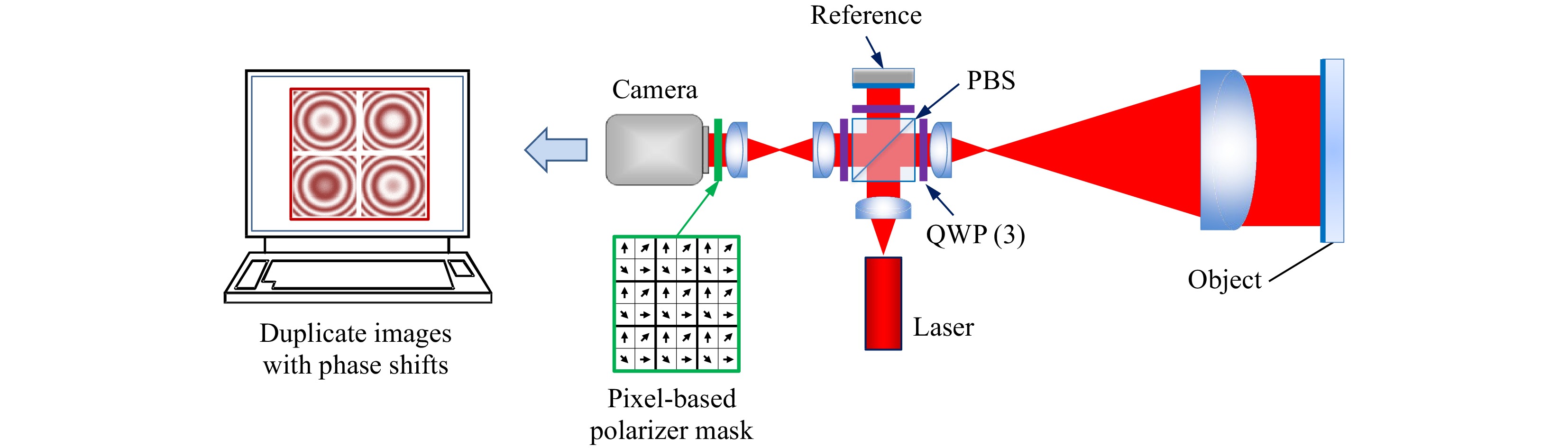
Fig. 4  Modern polarization-based phase shifting interferometer.

As is well known, the PSI concept is not limited to the simultaneous imaging of multiple interference patterns using polarization. Gabor and Goss note in their 1966 paper about their quadrature microscope that “…photographs can be of course obtained in succession¹³.” This is the basis of temporal PSI, which has the advantage of nearly identical optical path for each of the multiple phase-shifted images, minimizing error sources. The milestone work in temporal PSI was that of Bruning, who in 1974 measured topography using interferometry and computerized sine-cosine fitting^{18, 19}, following foundational work at Perkin Elmer²⁰. After the introduction of commercial mechanical phase shifting systems in the 1980s (Fig. 5), there was a flourishing of developments in PSI algorithm design, that has been extensively reviewed^{21, 22}. Today temporal PSI methods include adaptive and iterative algorithms to account for environmental disturbances and opto-mechanical imperfections²³.

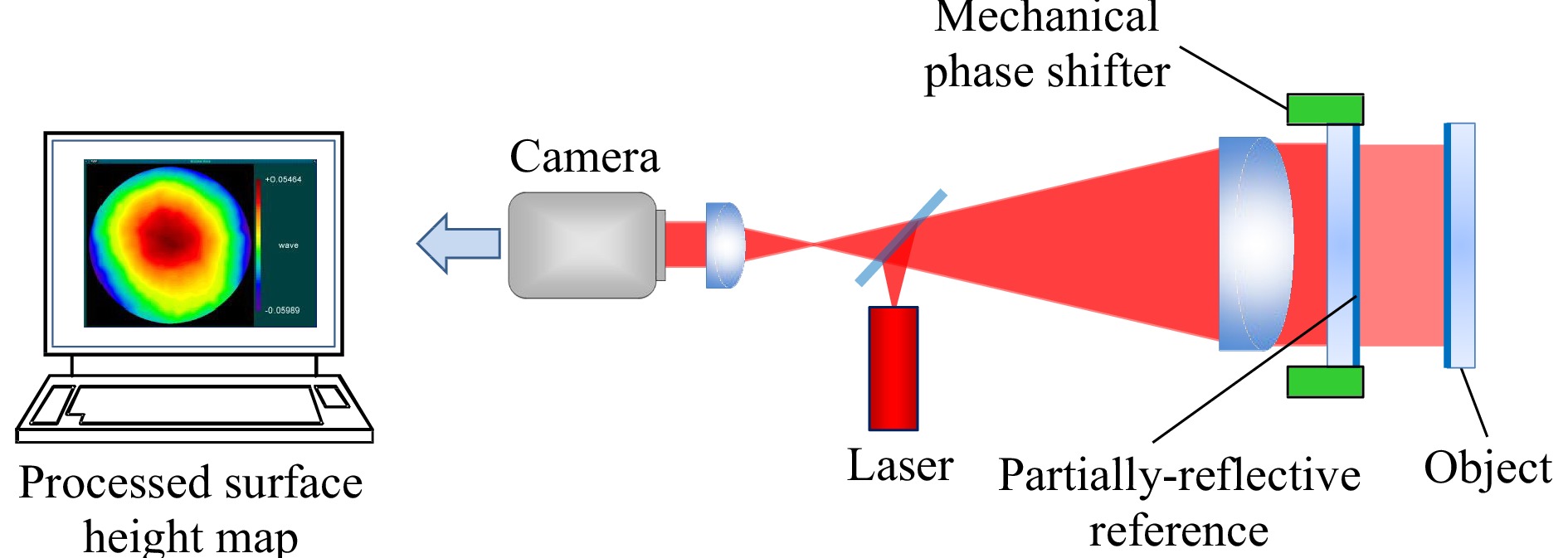
Fig. 5  Laser Fizeau interferometer with a mechanical phase shifting system for the reference flat.

The use of temporal PSI in holography developed along a parallel path to interferometry. Electronic phase evaluation of holograms in the 1970's included the work of Dändliker et al²⁴. However, true digital PSI analysis of holograms had to wait until camera pixel densities were sufficient to resolve the dense fringe patterns of holograms captured far from the in-focus image of the object surface Many advances followed developments of electronic speckle-pattern interferometry, dual-exposure holographic interferometry, and non-destructive testing, all of which are closely related to holography^25-27. These fields contributed significantly to determining the interference fringe order using phase unwrapping techniques developed for noisy speckle patterns²⁸.

Today both temporal and polarization-based PSI are employed for optical testing and interference microscopy, as illustrated by the large-aperture, wavelength-tuned PSI system of Fig. 6. While many factors contributed to its development, it can be meaningfully argued that many of the foundational ideas date back to the earliest work in wavefront synthesis using multiple phase-shifted holograms.

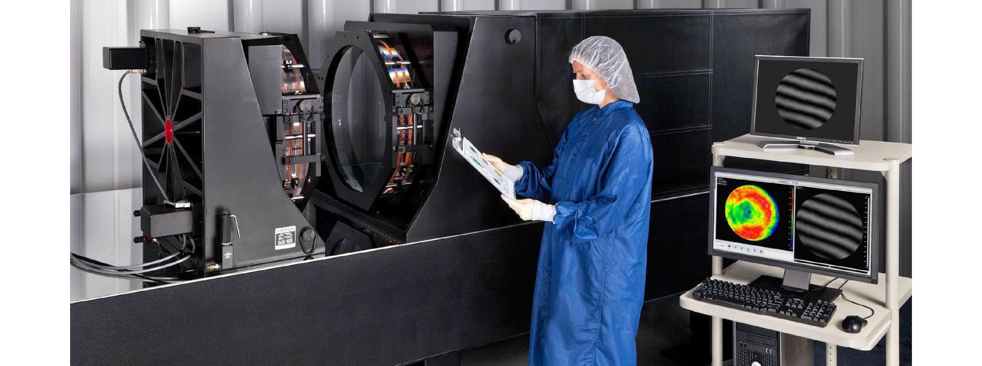
Fig. 6  A 600 mm aperture, wavelength-tuned, temporal phase shifting Fizeau interferometer for testing large optical flats. Photograph courtesy of Zygo Corporation.

A key breakthrough in holography came when Leith and Upatnieks showed that the overlapping images in Gabor holograms could be separated by using a reference wave at a large enough angle that the reconstructed real and conjugate images formed by the hologram become separable in the far field²⁹. This is illustrated in Fig. 1b, where $\alpha $ is this all-important diffraction angle. The result is equivalent to a single-sideband detection by optical methods³⁰.

By the 1970s, it was realized that the equivalent of far-field separation of the propagating wavefronts could be emulated for interferometry without holographic reconstruction. In the context of improving astronomical images, Roddier and Roddier analyzed wavefronts using direct electronic processing of carrier-fringe interferograms³¹. The concept gained popularity with the seminal work of Takeda in 1982, who described carrier fringe methods for structured light and interferometric measurements of surface topography. In spite of continuous improvements^{32, 33}, for many years the available computers and cameras were not quite up to the task of providing high lateral resolution images quickly using digital Fourier transforms. Mertz³⁴ and then Freischlad and Küchel³⁵ developed convolution kernels to speed up the calculations; but the carrier fringe technique was overshadowed in the 1990s by developments in temporal PSI. By the 2000s, enabling technologies had advanced enough for real-time data processing using two-dimensional digital Fourier transforms at high lateral resolution, and the carrier fringe technique was given new life³⁶.

The principle underlying carrier fringe methods in interferometry follows from communications theory and Lohmann's Fourier analysis of the holographic reconstruction process³⁰. To clarify this principle mathematically, we first introduce a nonzero tilt angle $\theta $ in the $ y,z $ plane defined in Fig. 1 for the reference light $ {u_R} $, such that Eq. 3 now reads

where

is the spatial frequency of the resulting carrier fringes in the interference pattern. If we simulate a holographic reconstruction with a plane reference wave of unit amplitude and zero phase, the scattered light can be represented by a spectrum $ \widetilde U $ of plane waves, each of which is the solution to the free-space Helmholtz equation^{37, 38}. The spectrum for this intensity pattern is

which we write as a Fourier transform

In the $ y,z $ plane, the Fourier frequency $ {f_y} $ corresponds to the diffraction angle $ \alpha $ according to

From Eq. 12 and 15, we have for the reconstructed light field in frequency space

In the far field, whether it is physical or a digital reconstruction in a computer, these three terms are separable by their frequency. It comes as no surprise given Fig. 1 that the last term, which contains the desired information and is centered at a spatial frequency $ {f_y} = \nu $, diffracts at an angle $ \alpha = \theta $. After isolating this last term and recentering it about zero frequency, the inverse transform is

If the reference light $ {u_R} $ has a uniform phase and intensity, or at least if it is known and can be compensated, this process recovers the original complex object field $ {u_0} $, with separable phase and intensity. Importantly, while the classical holographic reconstruction method involves illuminating the recorded pattern a second time with the reference light $ {u_R} $, this step is not required if we have a digital recording of the intensity $ I $ with sufficient lateral resolution.

In conventional interferometry, we assume that the optical system creates an imaged light field $ {u_I} $ that is as much as possible an in-focus duplicate of the object light field $ {u_o} $⁸. Because of the suppression of one of the sidebands in frequency space, the digital processing results in complex-valued light field $ {u_I} $, from which we readily determine the phase

and corresponding measured surface heights

Fig. 7 summarizes this sequence, from carrier-fringe interferogram to final topography map.

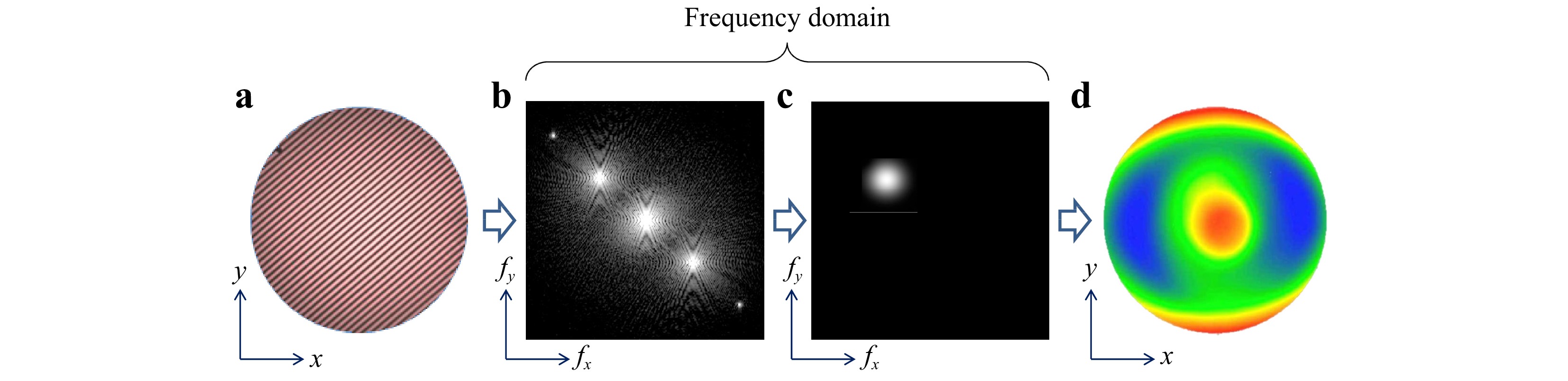
Fig. 7  Data processing for carrier fringe interferometry. a Original hologram with high density carrier fringes. b The two-dimensional Fourier transform of the hologram. c Frequency-domain filtering to isolate one of the Fourier sidebands. d The final surface topography map.

Fig. 8 illustrates a common configuration for creating dense carrier fringes in a Fizeau interferometer. A relative tilt of the reference and object surfaces results in dense interference fringes at the camera, on the order of hundreds of fringes over the viewing aperture. Provided that the instrument has manageable or compensated aberrations when operated off axis, this holographic data acquisition requires few changes in the opto-mechanical hardware of a laser Fizeau system. For this reason, carrier fringe interferometry is often option for systems that also offer mechanical phase shifting as in Fig. 5.

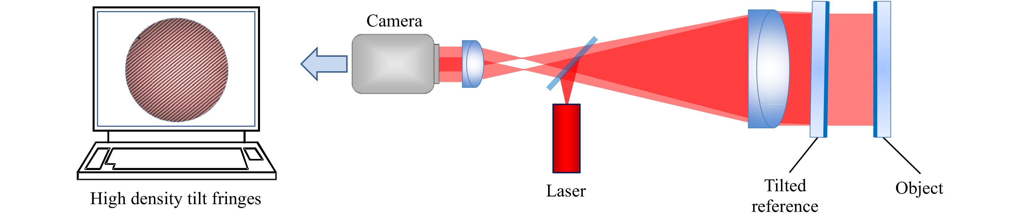
Fig. 8  Laser Fizeau interferometer configured for off-axis, carrier fringe interferometry.

Major advances in holography date from the invention of visible-wavelength lasers^{39, 40}. However, there are good reasons for not using lasers in holography and interferometry, because of speckle effects and coherent noise from dust particles and unwanted reflections⁴¹. Leith notes a benefit of arc lamps to reduce the noise in holograms, describing pre-laser experiments from 1958 to 1962 as “…quite a phenomenal success.”⁴² Line sources that are incoherent in one direction and limited coherence in the other substantially reduce the noise in carrier fringe holograms of flat objects²⁹.

With the arrival of the laser, it was possible to produce holograms of three-dimensional objects such as the chess piece in Fig. 1. The results provided astonishing depth and parallax, in a way that would have been impossible with previously-available light sources. Lasers enabled the wide range of holography applications that we know of today; but they came with new problems associated with increased coherent noise.

Even prior to the laser, Kirkpatrick and El-Sum noted in 1956 that with coherent imaging “…careful cleaning of the optical surfaces was found to remove only a minority of the noise sources... The whole nuisance was removed by rotating the entire light-source unit, including the filter, in a continuous manner about the optical axis of the system.”⁴³ If the time of exposure is long, these motions reinforce the desired stationary pattern while averaging away much of the coherent noise^44-47. Averaging may be achieved in different ways, including rotating an optical element around the axis of the optical system, moving a diffuser across the illuminating beam, changing the incident direction of the illuminating beam with a rotating element, or by moving different masks in the Fourier plane of the imaging system^{48, 49}. Fig. 9 illustrates a method proposed by Close in 1972 for a portable holographic microscope based on a pulsed ruby laser⁴⁶. The microscope records four holograms, each with an independent speckle pattern corresponding to a rotary position of the prism. The four images formed by the holograms are incoherently superposed to reduce coherent noise and speckle granularity.

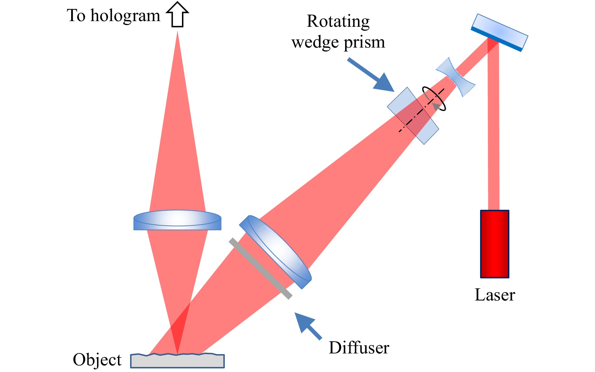
Fig. 9  Coherent noise reduction system using a rotating wedge prism.

The diagram shows only the illumination of the object—the reference path is separate.

Lasers began to appear in unequal-path configurations in the 1960s⁵⁰, and averaging methods originally developed for holography to reduce coherent noise were shown to be effective for improving results in interferometry⁵¹. Fig. 10 illustrates the averaging technique applied to a Fizeau interferometer^{52, 53}. In this example, each surface height map is the result of a single camera frame data acquisition using the tilt-fringe method^{54, 55}. Between each acquisition, the direction of illumination by the laser light source is changed by eccentric rotation of a lens near the system focus of the Fizeau geometry. The left-hand surface topography image in Fig. 10a shows high-spatial frequency coherent noise that moves depending on the position of the light source. The average of 16 height maps shown in Fig. 10b for a continuous change in source position is smoother and a better representation of the true surface topography, with much reduced coherent noise.

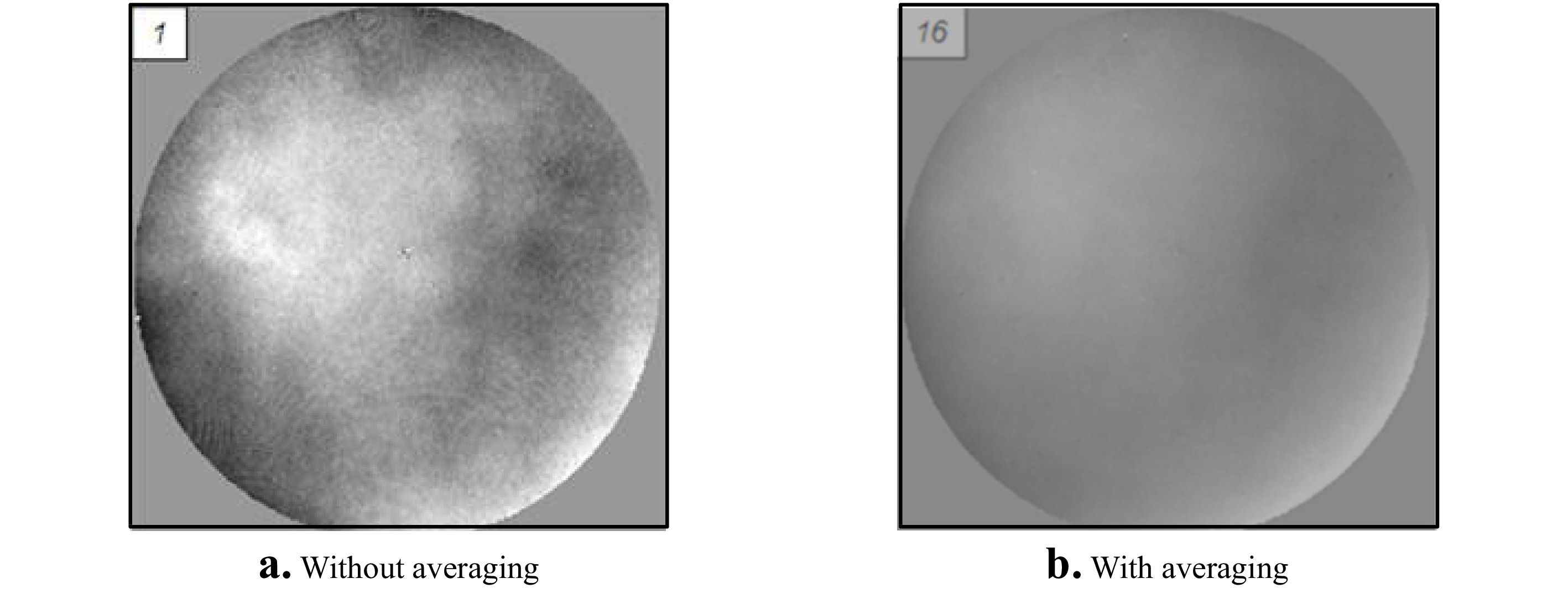
Fig. 10  a: Grey-scale surface height map by reconstruction of an object surface topography from a single camera frame using carrier-fringe methods. b: Improved image quality after averaging 16 topography maps with the light source rotated about the optical axis between data acquisitions. The surface height range for these images is a few nanometers.

In place of averaging final topography maps, an alternative method for coherent noise reduction is to synthesize a larger monochromatic source size in real time, using a laser in combination with rapidly-rotating mirrors or diffusing disks. An advantage is that the ‘live' camera image is itself improved, and data averaging is not necessary. A basic requirement is that the coherence reduction should not adversely affect the interference fringe contrast, sometimes leading to an adjustable apparent source size⁵⁶. An effective means of preserving fringe contrast with an extended source in a laser Fizeau was invented by Küchel, based on tracing a point source in a circle or ring about the optical axis, which preserves the desired interference fringe pattern while randomizing other coherent effects⁵⁷.

In some instruments the reduction in coherence follows a fully coherent portion of the optical system. Commercial Fizeau interferometers often employ coherent imaging to project an interference pattern onto a rapidly-rotating diffuser, resulting in randomized speckle, before a multi-element zoom lens creates the final image on the camera⁵⁸. The benefit is high interference contrast, without coherent artifacts and patterns from the imaging optics and camera cover slips. With the advent of large-format cameras, however, the higher lateral resolution of fully-coherent imaging has made it more attractive to directly image onto the camera⁵⁹.

Gabor's background and research interests led him to think of holography as a new microscopic imaging technique with a large depth of field, allowing the microscopist to examine the different planes of the image at leisure². The ability to refocus the image after it is recorded remains one of the defining characteristics of holography, and frees us from the need to carefully image objects onto film or a detector. It also enables the recording of measurement volumes, with the ability to sharply image cross sections of three-dimensional data⁶⁰. The capability became even more attractive with digital holography, for which the refocusing is achieved entirely within a computer⁶¹.

The process of digitally refocusing is straightforward, provided of course that we have knowledge of the object light field $ {u_0} $, gained by holographic reconstruction or by high-resolution digital interferometric recording with PSI or carrier-fringe analysis. To evaluate how this light propagates, as before, we first determine the spectrum of plane waves from the Fourier transform

As the light propagates in the $ z $ direction, the spectrum of plane waves evolves according to

where the free-space propagator

accounts for how much each plane wave will be shifted in phase in terms of a distance $ z $. The inverse Fourier transform is the focus-shifted object light field:

These calculations are astonishingly powerful, enabling in some cases the recording of images without any imaging optics—the focusing and real or virtual image formation is performed afterwards in a computer. Hence one of the popular definitions of holography as lensless photography⁶².

Although digital refocusing is familiar in digital holographic microscopy⁶³, it is not usually considered a feature or capability of surface-topography interferometry. Nonetheless, from the preceding mathematical description of the method, it is entirely feasible to refocus conventional interferometry data in the same way after acquisition. As data densities have increased, so has interest in correcting for focus errors to maintain high lateral resolution in interferometry.

Unlike holographic systems, traditional interferometers are arranged such that the object surface is precisely focused onto the camera prior to data acquisition. Fig. 11 illustrates a simplified focus mechanism. Focusing is often a manual process, involving a subjective determination of image sharpness. Because optical surfaces are often featureless by design, a common procedure involves positioning a straightedge as close as possible to the adjusting surface and adjust focus until the straightedge appears sharpest. The combination of cumbersome setup and human error are such that it is reasonable to assert that very few interferometers today are operating at their full potential, simply because of focus errors. Digital refocusing presents an opportunity to solve this problem using software.

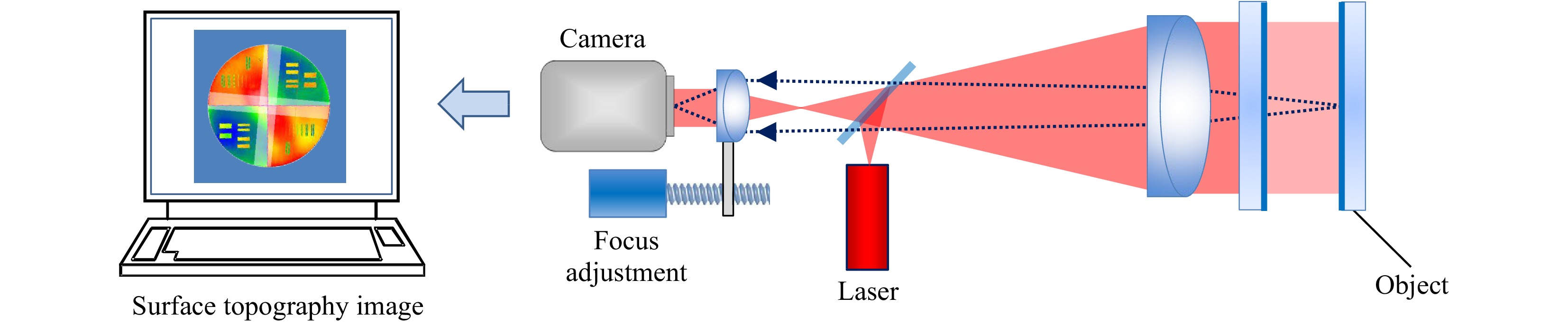
Fig. 11  Focusing mechanism for a laser Fizeau interferometer.

To evaluate the benefits of digital holographic refocusing in an interferometer, we first need to define what is meant by lateral resolution. Some familiar examples include the widely-known Rayleigh and Sparrow limits, which in conventional greyscale imaging correspond to the smallest separation between object points for which there are two clearly separable image points⁶⁴. A frequency-domain equivalent is the Abbe limit, which is the highest detectable sinusoidal spatial frequency. These limits have analogous definitions for surface topography measurement⁶⁵. However, it has become common to quantify topographical lateral resolution by means of the instrument transfer function (ITF), which describes an instrument's height response over a range of spatial frequencies^{64, 66}. The ITF formalism has several limitations, including the requirements of linear height response and shift invariance, but it nonetheless provides a more complete description of lateral resolving power than a single number⁶⁷.

The most favorable ITF is achieved at the position of best focus. Fig. 12 shows experimental results for two different focus positions showing the sensitivity of ITF response to focus error. The ITF evaluation consists of a Fourier lateral spatial frequency analysis of the edge spread function, using a specialized ITF artefact with embedded topographical step features. What is most notable about these results is they represent two distinct outcomes for what appears to be nearly identical image sharpness, as shown in Fig. 13. The reason for this is that the higher spatial frequencies—those from 9 to 10 cycles/mm—present the identical impression of sharp edges in a subjective test. A consequence is that a traditional focus adjustment using the eye in place of a complete evaluation of the ITF can easily result in setting the incorrect focus.

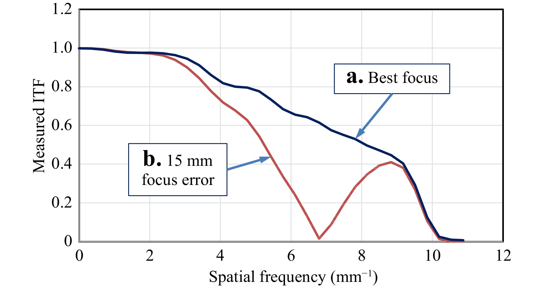
Fig. 12  Height response of a laser Fizeau interferometer as a function of surface spatial frequency for two different focus positions: a Best focus. b Object surface out of focus by an amount equivalent to moving the object axially 15 mm away from best focus.

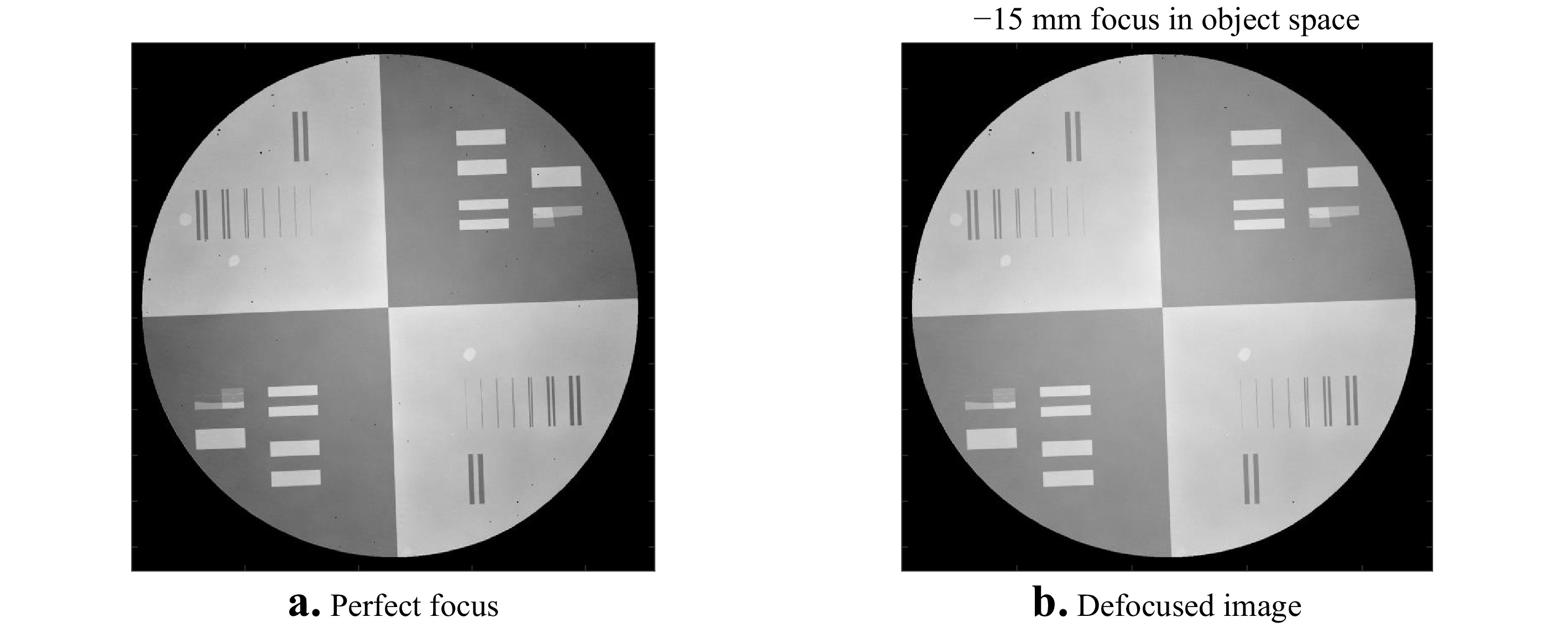
Fig. 13  Greyscale topography images with a surface height range of 50 nm for a 100 mm diameter ITF artefact, for the two difference focus positions a and b, shown in Fig. 12.

The results shown in Fig. 12 motivate the use of digital holographic refocusing to automate the focusing process⁶⁸. Propagating the complex-valued interferogram in object space and integrating the ITF curve for each position results in Fig. 14. In this case, the best focus position is approximately 15 mm away from the initial setup. Using this information, an encoded mechanical focus system readjusts the interferometer to the position that provides the best possible lateral resolution, as defined by the ITF and the closely-related Strehl ratio. There remains only to have an automated way of locating the physical location of an object that does not have any surface features—a task that is readily accomplished using a wavelength-tuned laser source to calculate the distance from the reference surface to the object surface⁶⁹.

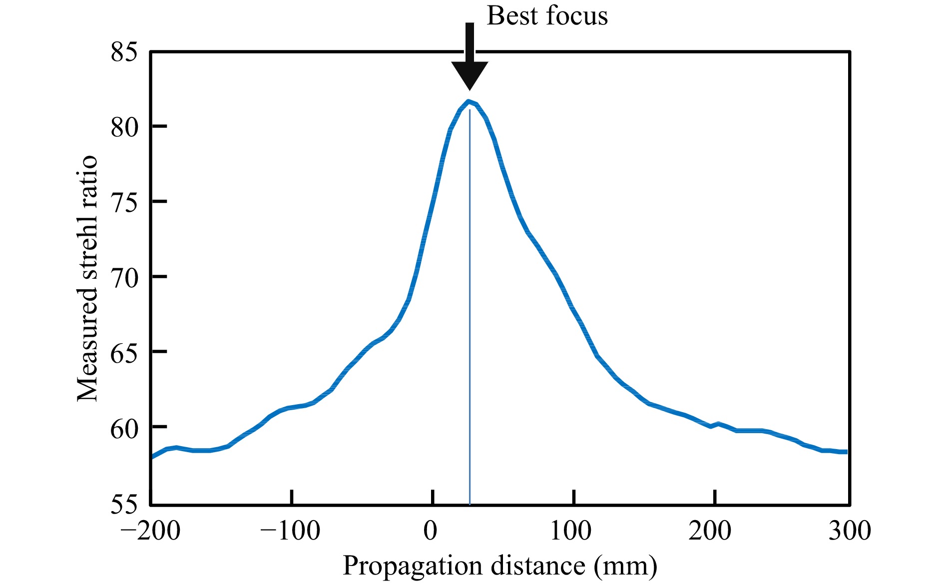
Fig. 14  Integrated ITF values as a function of focus position, obtained with digital holographic propagation in software.

While it is certainly possible to focus the system shown in Fig. 11 without digital holography, this is only because there is a single object with a surface shape that is well within the depth of field. Modern laser Fizeau interferometers are capable of measuring multiple surfaces in an optical system simultaneously using frequency-domain PSI methods⁷⁰. Fig. 15 illustrates this capability. In place of a mechanical or polarization-based phase shift, the laser source is swept in optical frequency by an amount $\Delta \nu $, resulting in a phase shift $ \Delta \varphi $ for the interference fringe pattern given by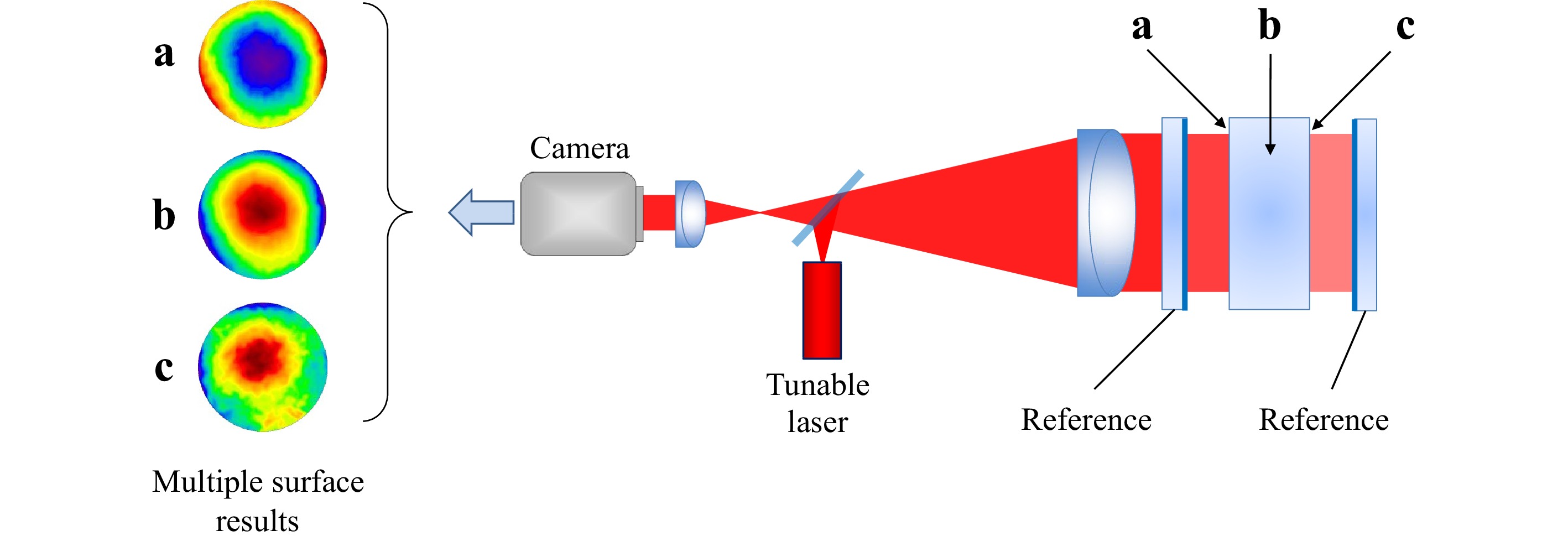

Fig. 15  Multi-surface testing using a wavelength-tunable laser and frequency-domain PSI for measuring a the front surface, b the material homogeneity and c the back surface of an object or optical system.

where $ L $ is the group-velocity optical path distance to one of the object surfaces, and $ c $ is the speed of light. Tuning the laser isolates the signal contributions of each of the object surfaces based on the size of the phase shift as a function of the frequency sweep according to Eq. 25. The phase shifting also enables the reconstruction of the topography for each individual surface⁷¹. However, for multiple surface testing with a single data acquisition, the best focus position varies with each surface. Thus digital holographic methods are essential to refocusing the extracted interferograms after data acquisition⁷². In this instrument, there is a true fusion of the two measurement principles in what can best be described as a digital holographic Fizeau interferometer.

If he were alive today, Isaac Newton might claim to have been the first person to have captured a hologram experimentally—as a drawing—as well as to have provided a formula for synthesizing a hologram computationally for a variety of wavelengths. The evidence is a drawing in the 2^nd book of “Opticks,” illustrating the famous experiment that we recognize today as the Newton's rings, formed by the interference of light reflected from a convex lens in contact with a flat glass plate⁷³. Hooke might also make a claim of priority if he were alive today, as previous to Newton he had observed a similar effect, and unlike Newton, was open to the idea that the phenomenon could be understood in terms of light waves⁷⁴.

To see how the experiments of Hook and Newton relate to the modern technique of computer-generated holograms to assist in interferometry for surface topography measurement, we must advance in time to Gabor's discovery of holography. One of the obstacles to the early acceptance of ‘diffraction microscopy' as a promising idea was the difficulty in understanding the theory behind the technique conceptually. In the absence of the compelling demonstrations of 3D images of toy trains and chess pieces that were not technically feasible without a laser, the holographic principle initially had to be appreciated at a theoretical level. The now familiar maths seemed esoteric and inaccessible, even to many physicists⁷⁵. To facilitate understanding of the new method, Rogers in 1950 proposed a conceptual approach in which a Gabor hologram is thought of as a superposition of Fresnel zone patterns, each one of which forms an image point⁷⁶. These individual patterns look very much like Newton's rings, as illustrated in Fig. 16.

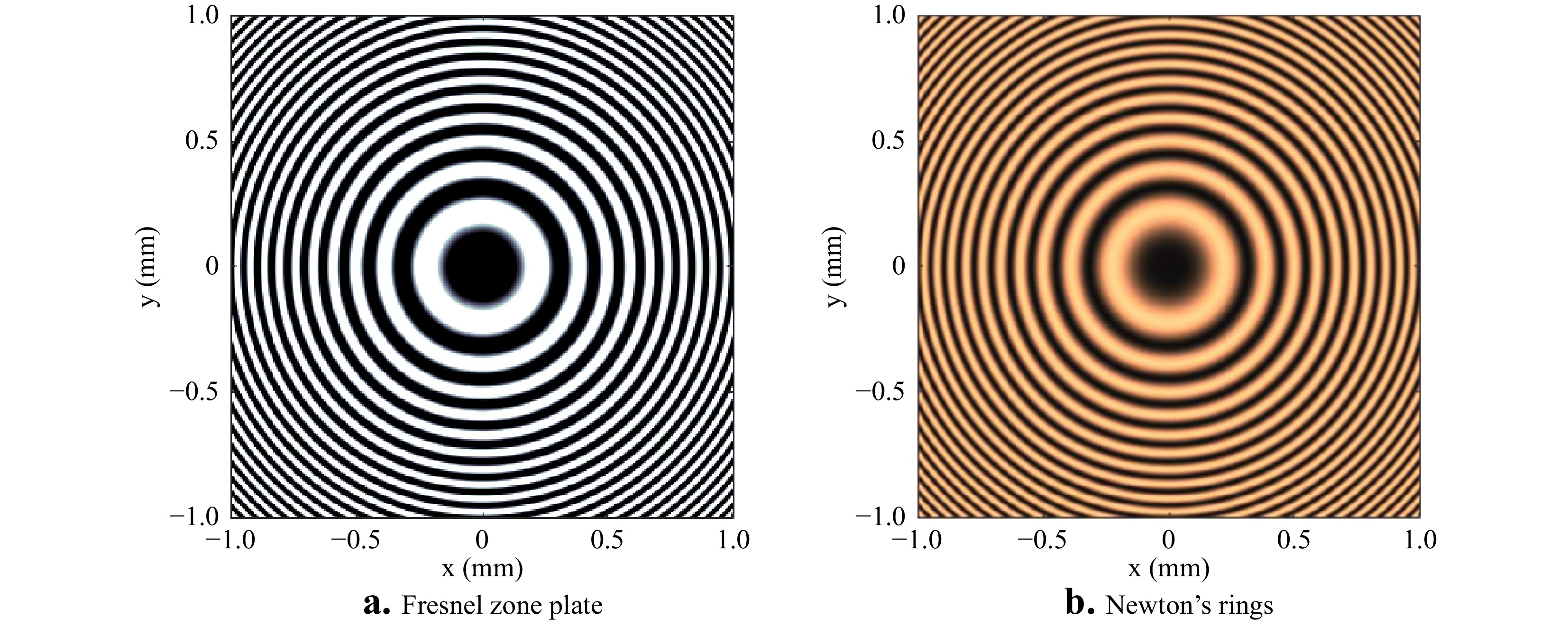
Fig. 16  a Computed Fresnel zone plate pattern for creating a focus at a distance of 100 mm at a wavelength of 0.5 $ \mu m $. b Newton's rings at the same wavelength for a convex surface with a radius of 200 mm in contact with a flat reference surface, equivalent to a Gabor hologram of a single virtual source point.

Fresnel zone patterns on glass plates have been familiar since the time of Rayleigh in the 19^th century as an elementary kind of diffractive optic⁷⁷. An analysis for the radius $ \rho $ of the alternating bright and dark circular zones readily leads to the formula

where $ R $ is the distance from the plate to the focal point, and $ m $ is the integer index for the alternating zones⁷⁸. This formula, not coincidentally, is nearly identical to the formula for the alternating bright and dark interference fringes in Newton's experiment:

where the distance $ R $ is the radius of curvature of a convex spherical surface in contact with a flat glass, and the factor of 2 difference is the result of viewing the spherical glass in reflection. A photograph of Newton's rings is therefore equivalent to a Gabor hologram of a single image point. The humble zone plate therefore shares many of the essential characteristics of holograms, including that any portion of the zone plate can be used to create a focus spot. In Newton's drawing, for example, only half of the ring structure is represented, which has a similar pattern to that of a Leith-Upatnieks off-axis hologram for a single image point³⁰.

These analogies between zone plates and synthesized or computer-generated holograms (CGHs) were well understood by researchers developing applications for new laser-based, unequal-path interferometers for testing the surface form of optical component in the late 1960s. The driving force in these developments was the need for accurate testing of lenses and mirrors having aspherical surface form. Twyman argued already in 1918 in favor of the increased use of aspheres in optical designs, recognizing that with the aid of an interferometer “…the optician can face without dismay the task of making with precision quite considerable departures from the sphericity…”⁷⁹ However, interferometers are best configured as null detectors, providing the highest precision and accuracy when comparing object and reference wavefronts of nearly identical shape. While there are many clever ways to achieve a null test using reflecting and refracting optics for specific species of asphere, such as those represented by a single conic constant, the CGH dramatically increases the solution space by simply altering the formula for the opaque and transparent zones⁸⁰.

One of the attractive features of CGH null correctors is that the accuracy of wavefront construction is largely determined by the in-plane location of the diffracting zones, rather than surface heights. Thus, in place of painstakingly polishing an aspherical reference surface to nanometer precision, it is possible to synthesize the reflected wavefront from a precision reference on a more relaxed dimensional scale. In 2007, in a fascinating retrospective of the early days of CGHs, Lohmann describes the use of pen plotters and hand touch-up in the 1960s to create simple grey-scale patterns that were photographically reduced to usable holograms⁸¹. These experiences with pen plotters and ruling engines for CGHs were duplicated or independently reinvented in several labs worldwide. By the 1970s, pioneering work by Pastor⁸², Wyant⁸³, Schwider⁸⁴, and many others rapidly filled in the configuration and application space for CGH-compensated interferometers for optical components^{85, 86}. The development of advanced photolithography and electron beam writing for semiconductor manufacturing has led to present-day capabilities for testing optics using a configuration similar to that of Fig.17 with far greater departure and higher accuracy than Twyman would have imagined possible⁸⁷.

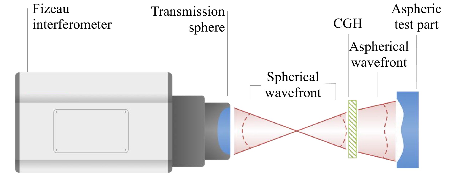
Fig. 17  Configuration for optical testing of an aspheric surface using a laser Fizeau interferometer with a CGH.

The CGH technique for optical testing has received significant competition from methods that seek greater flexibility than can be provided by a null test. Methods involving axial scanning for rotationally symmetric aspheres, when provided with precision staging systems, achieve uncertainty levels approaching those of custom CGH solutions without a fixed optical configuration for each part type⁸⁸. Reconfigurable geometries based on spatial light modulators assemble zones of low fringe density into final topography maps using a sequence of off-axis illumination angles⁸⁹. Another solution is an optical stylus with precision part motions to trace out full 3D topographies with single-point scanning⁹⁰.

To remain competitive, developers have leveraged advances in enabling technologies to make CGH solutions more accessible and practical for fast, production-line testing with simplified part alignment. Fig. 18 illustrates modern use of a CGH for aspheres and freeforms. The instrument is an upward-looking, 633 nm wavelength laser Fizeau, and the test part is a diamond-turned, rotationally symmetric asphere with a radius of 128 mm for the best fit sphere. The aspheric departure is 70.8 µm over a 44 mm diameter. The off-axis, lithographically-produced, binary CGH is positioned just below the part. The CGH and the part are held in precision kinematic fixtures shown in Fig. 18a that allow for part removal and replacement without realigning the instrument to achieve the low fringe density shown in Fig. 18b. The final height map in Fig. 18c shows that the part deviates from design, with a residual 0.223 µm peak-valley (PV) central feature at this stage of machining, after compensating the 70.8 µm departure using the CGH.

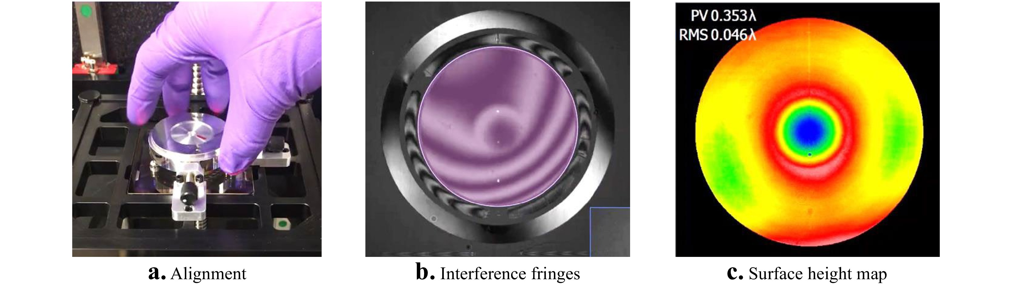
Fig. 18  Modern example of a CGH or diffractive-optic null corrector for a testing an asphere. Photographs courtesy of Zygo Corporation and Arizona Optical Metrology (AOM).

The most obvious contribution of holography to interferometry is clear from the name of the technique: ‘holographic interferometry.' This discovery by several researchers working in laser-based 3D imaging holography in the mid-1960s ushered in a wide range of applications of high interest to metrologists^{91, 92}. The term ‘discovery' applies perfectly here, as many of the first steps towards this powerful technique were taken experimentally, sometimes by accident, and later explained theoretically^{93, 94}. There are now many books on the subject, cataloguing methods for quantitative analysis of stress, strain, deformation and overall contour of diffusing objects rendered in 3D by means of holography^95-98.

As we shall see in this section, the discovery of holographic interferometry has had a profound influence on capabilities and interpretations of interferometric techniques⁶. To identify and examine these connections, it is useful to follow the conceptual approach of Heflinger et al. in their 1966 paper on what was at that time the new field of holographic interferometry⁹⁹. We first consider a flat object that is tilted between two holographic exposures of the same hologram. Fig. 19a shows a simulated hologram with the dense carrier fringes characteristic of off-axis holography of plane objects with collimated reference and object illumination. This is sometimes referred to as the “primary image” in holographic interferometry. Fig. 19b illustrates the effect of a double exposure, with the object tilted slightly along a diagonal between exposures. The incoherent superposition of the intensity patterns for the two object orientations results a modulation of the fringe contrast in the hologram, that we readily perceive by eye. When this double-exposure hologram is reilluminated with the reference wave to synthesize the original wavefront from the object, the result is a fringe pattern as shown in Fig. 19c, superimposed on the object image¹⁰⁰. The fringes in Fig. 19c are the result of variations in diffraction efficiency attributable to the contrast modulation in the hologram⁹⁹. The orientation and density of the fringes informs us how the object has changed between exposures. In this case, the object has been tilted along a diagonal without deforming the object surface, resulting in straight fringes, the density of which is a measure of the amount of tilt.

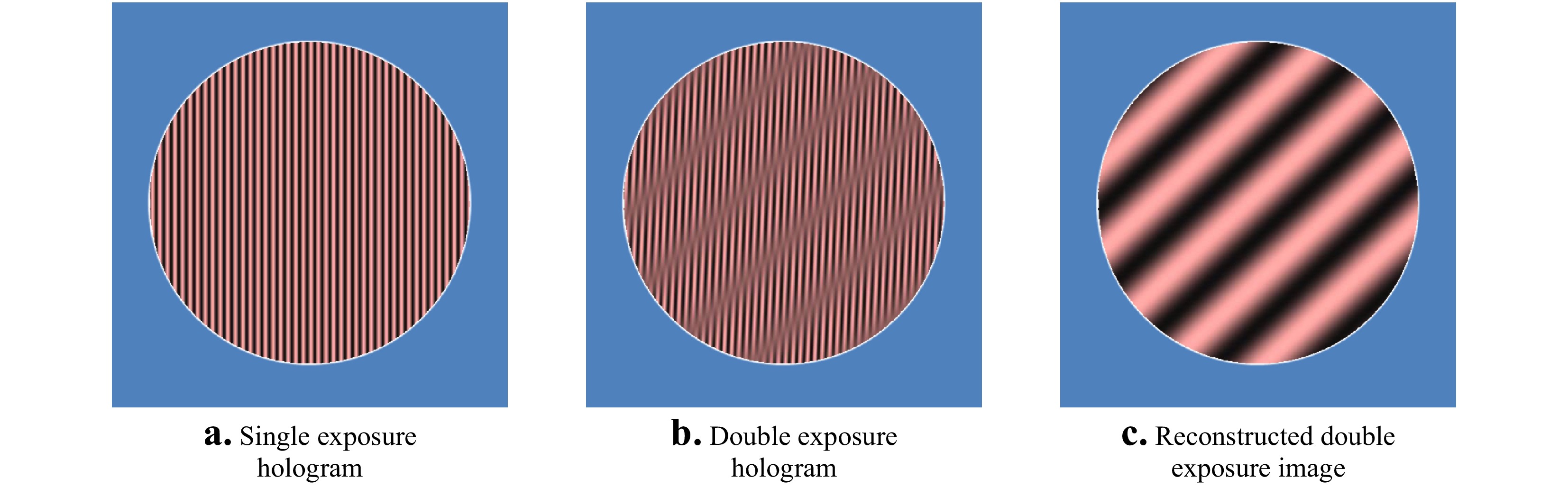
Fig. 19  Simulations illustrating double-exposure holography for a flat part. a Carrier fringes resulting from a single off-axis exposure with collimated light; b incoherent superposition of two exposures with slightly different tilt angles for the part; c the result of creating a part image from the double-exposure hologram by wavefront synthesis.

In the example of Fig. 19, we see that the holographic recreation of a propagating wavefront serves to demodulate the incoherent superposition of interference patterns present in the double-exposure hologram, converting contrast variations to interference fringes representing the difference between the two exposures. Since these superimposed patterns in the hologram are mutually incoherent, they can be generated at different times, with different positions for the component parts of the holographic system, and even with different wavelengths. Hence the astonishingly wide range of applications for the technique.

An intriguing interpretation of holographic interferometry is the concept of temporal wavefront division. When the hologram of Fig. 19b is illuminated with coherent light, the reconstructed wavefront from the first exposure interferes with the wavefront from the second exposure, resulting in the interference pattern of Fig. 19c, even though the exposures were captured at different times^{94, 99}. A compelling example of this interpretation is the presence of ‘live' fringes from a single-exposure hologram with the object illuminated once again and viewed through the hologram. In this case, the fringe formation takes place dynamically, revealing deformations caused by varying loads, vibrations and temperature gradients in real time, by detecting the minute differences between the original exposure and the light reflected from the object⁹³.

The many extraordinary capabilities of digital holographic methods would seem to be unique to holography. However, there is a link to conventional interferometry in the fringe contrast modulations in image-plane holograms. The effect of a double exposure on a hologram is an interference pattern that can be directly interpreted without the need to recreate propagating wavefronts according to the second step (b) shown in Fig. 1 of a holography experiment⁹⁹. In their 1965 paper on vibration analysis using wavefront reconstruction, Powel and Stetson credit Osterberg for a method developed in 1932 for visualizing the resonant mode analysis of quartz crystals using a Michelson interferometer^{101, 102}. The contours of the resonant modes in the Osterberg experiments appear as fringe contrast patterns that are interpreted with exactly the same Bessel function analysis used in holographic interferometry.

After the discovery of holographic interferometry, Polhemus¹⁰³ developed in 1973 a Twyman Green two-wavelength interferometer using analog electronic demodulation to generate an equivalent-wavelength fringe pattern that follows the surface shape, similar to a double-exposure holographic setup, but without the step of illuminating the hologram and observing the diffraction patterns. In 2003, Bosseboef and Petigrand¹⁰⁴ and Patorski et al¹⁰⁵. developed methods using a conventional phase shifting interference microscope to demodulate the fringe contrast contours for resonant mode analysis of micro-machined parts. There are many such examples, where demodulation of complicated interference patterns emulates the functionality of holographic interferometry without the physical reconstruction of wavefronts by coherent illumination of holograms.

An interesting and unexpected example of how holographic techniques and signal analyses have informed developments in optical metrology is coherence scanning interferometry (CSI), currently the most widely-used method of interference microscopy for measurements of surface topography^{106, 107}. The CSI instrument shown in Fig. 20a uses spectrally broadband light and high numerical apertures to generate fringe-contrast variations in the interference pattern shown in Fig. 20b. In a similar way to holography, the interference image is essentially indecipherable, even though the rough object surface is in focus. To make sense of the interference information, the pattern must be demodulated, so as to separate contrast effects from the fringes themselves. In his 1984 PhD thesis, Haneishi¹⁰⁸ adapts the digital holographic carrier-fringe signal processing method described by Takeda⁵⁴ for analysis to these CSI fringes. The method relies on scanning the interference objective axially so as to create a signal similar to the one shown in Fig. 21a for a single image point or camera pixel. This signal is Fourier transformed along the $z$ scanning direction to the frequency domain, where the positive-frequency sideband is isolated and shifted to zero frequency prior to inverse transforming to create a new signal corresponding to the fringe contrast envelope alone. Tracing the peak value of the fringe contrast over the field of view creates a topography map similar to the one shown in Fig. 21b. Although software procedures have evolved significantly and independently from holographic interferometry since 1984, a frequency domain analysis of CSI signals is the foundation for many advanced CSI systems today^{107, 109}.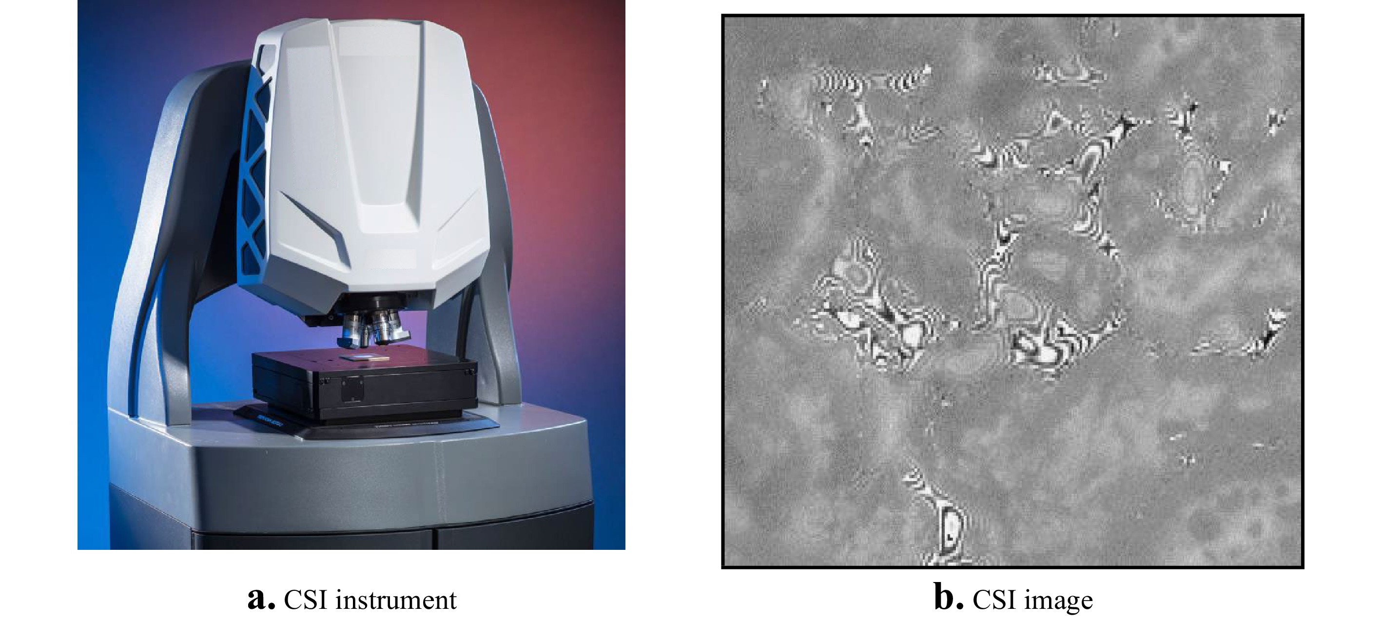

Fig. 20  a A coherence scanning interferometer based on a microscope platform. b A single camera frame image of an interferogram captured with this instrument, for a textured surface.

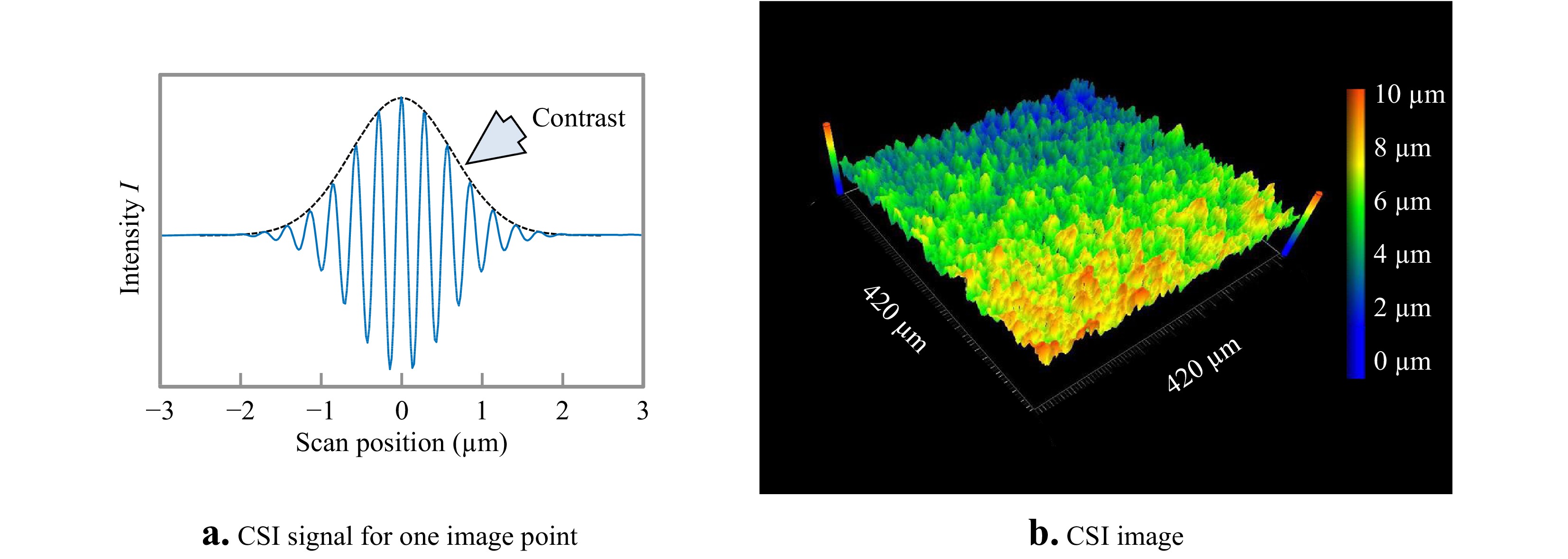
Fig. 21  a Simulated signal for one image point or camera pixel during an axial scan of the interference objective in a CSI instrument. b Experimentally measured topography corresponding to the interference pattern shown in Fig. 20b.

Holographic imaging of 3D objects, many of which are as deep as they are wide, presents a challenge for diffraction theories based on representing a wavefront as a complex amplitude distribution in an $ x,y $ plane propagating in the $ z $ direction. What, exactly, is the structure of a light field scattered from the chess piece in Fig. 1? How can it be represented within a plane, as we have done so far in this paper? When we reilluminate the hologram, how can we calculate the resulting 3D image? These questions about holographic recording and imaging stimulated in the 1960s a reevaluation of the theory of light scattering and imaging in 3D. In this section, we briefly review how holography has influenced the development of 3D diffraction theories for the evaluation and performance improvement of interference microscopes.

Many of the properties of optical instruments can be understood using tradition of Abbe theory and Fourier optics modeling, including the spatial-bandwidth filtering properties of imaging systems.^{37, 66, 110, 111} The first step in a Fourier optics model of an interferometer is to simplify the representation of the surface topography to a phase distribution confined to a plane normal to the optical axis^{112, 113}. The most common approach is to assume a linear relationship between the surface height at the measured phase shift, as in Eq. 9

from which we calculate the complex-valued object light field in the $ x,y $ plane using Eq. 1

In effect, the surface topography is imprinted upon the reflected wavefront as a variation in phase $ {\phi _o} $ proportional to the surface height $ {h_o} $. The corresponding spectrum of plane waves follows from Eq.(21):

To account for the filtering effects of imaging, classical Fourier optics defines a frequency-domain transfer function (TF) $ \widetilde H $, resulting in an imaged spectrum $ \widetilde {{U_I}} $ :

The simplest transfer function for coherent imaging is a simple frequency bandwidth limit based on the NA $ {A_N} $ of the imaging system:

where in this case the Abbe frequency is

The imaged light field is then

In most interferometry applications, we consciously ignore the effects of optical filtering and field-dependent focus effects and write

where the phase

is determined by PSI or some other means of phase estimation based on interpretations of the interferograms created by mixing the imaged light field $ {u_I} $ with a reference light field $ {u_R} $.

A more realistic approach to the imaging problem begins by defining the object as a distribution of scattering points in volumetric space, as opposed to height values within an object surface that shift phase values in a complex representation localized to a plane. In 1967, Frieden described a transfer theory in terms of a 3D spectrum of plane waves scattered from such objects, and found that for both incoherent and coherent illumination, the image obeys linear frequency-domain theorems that resemble the familiar results of classical 2D Fourier optics¹¹². These theories were expanded in the context of holography by Wolf^{114, 115} and by Dändliker and Weiss¹¹⁶. These 3D Fourier methods are foundational for modern digital holographic microscopy^{117, 118} and quantitative phase imaging¹¹⁹.

3D imaging theory for non-holographic interferometry has followed a circuitous path¹²⁰. The traditional modeling of what is fundamentally a 3D problem using 2D complex representation of the object surface as in Eqs. 28,29 implicitly assumes that all surface points can be at the same focus position along the $ z $ direction at the same time. The limit to this 2D approximation is that the surface height variations must be small with respect to the depth of field of the imaging system^{110, 121}. For surface topography measurements using interferometry, this is not so challenging a limitation—common Fizeau interferometers have depths of field on the order of several millimeters and a surface height measurement range of perhaps a few 10s of micrometers. For this reason, adoption of 3D methods has been taken up more quickly in high-magnification microscopy, particularly for confocal microscopy, which works precisely on the principle that surface topography features at high NA cannot all be at the same focus position relative to the depth of field^{122, 123}.

While 2D Fourier optics is adequate for Fizeau interferometers with apertures of 100 mm or more, it is a less satisfying approximation for interference microscopy, for which the sharpness and contrast of interference fringes at high magnifications can vary with just a few micrometers in height variation¹²⁴. Coupland and colleagues have derived the 3D image formation and effective transfer function of CSI based on the Kirchhoff approximation where the surface of a homogeneous medium is represented as a continuous single layer of scattering points¹²⁵. This approach has been demonstrated to be of significant practical value, not only for understanding the origins of measurement errors as a function of slope, curvature, and focus^126-128, but for correcting aberrations as well¹²⁹.

Although 3D imaging theory for interferometry shares some common concepts with the 2D Fourier optics model, there are some significant differences. In place of the simple conversion from topography $h$ to phase-shifted wavefront in the $x,y$ plane as in Eqs. 28,29, the object surface is defined by a 3D Dirac delta function ${\Delta _o}$, which represents an infinitely thin scattering layer under the Kirchhoff approximation. The 3D Fourier transform of this surface model is:

or more compactly,

Importantly, this spectrum $ \widetilde {{\Delta _o}} $ does not contain any information at all about the optical system—it is a frequency-domain description of a representation of the object surface itself. All of the information about the optical system is contained in the 3D TF $ \widetilde {{H_{3D}}} $, defined as a linear, shift-invariant frequency-domain function that maps from the object directly to the interference fringes $ {O_I} $, which for two-beam monochromatic interferometry is the cosine part of Eq. 10¹³⁰. The corresponding 3D frequency representation is

from which we calculate

It can be shown that this 3D formalism duplicates classical 2D Fourier optics modeling if the object ${\Delta _o}$ is defined as a thin phase object contained entirely within the $x,y$ plane¹³⁰.

To gain insight into the geometrical meaning of 3D transfer functions, it is useful to work through the construction of a cross-sectional TF corresponding to the $y,z$ plane of incidence for monochromatic interferometry at high NA¹³¹. The construction starts in Fig. 22a by defining incident wavevectors ${{\bf{k}}_{\bf{i}}}$ and scattered wavevectors ${{\bf{k}}_{\bf{s}}}$. These wavevectors have a length given by the inverse wavelength ${1 \mathord{\left/ {\vphantom {1 \lambda }} \right. } \lambda }$. In an interferometer, the phase sensitivity to surface topography for a given pair of incident and scattered wavevectors is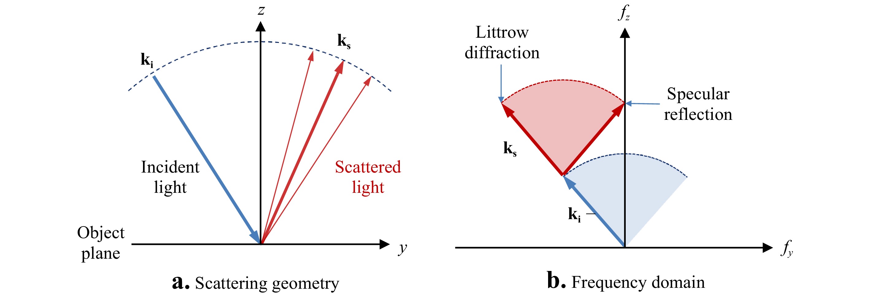

Fig. 22  a Geometry of incident and scattered rays at a surface. b The corresponding frequency domain illustrating the process of determining the range of possible spatial frequencies detected by the instrument.

This is illustrated in Fig. 22b, where the corresponding frequencies are

The range of possible ${{\bf{k}}_{\bf{i}}}$ orientations consistent with the illumination geometry sweeps out an arc. For each incident wavevector, there is a corresponding arc of possible scattered wavevectors ${{\bf{k}}_{\bf{s}}}$, limited by the acceptance cone of the imaging system. The combination of these two arcs defines the range of ${f_y},{f_z}$ values that are detectable using interferometry. Sweeping the ${{\bf{k}}_{\bf{i}}}$ and ${{\bf{k}}_{\bf{s}}}$ vectors through all possible angles results in a magnitude distribution proportional to the number of ways in which these vectors can be oriented to reach the same point in frequency space.

Fig. 23 shows the final 3D TF result for a spatially-incoherent, monochromatic light in an interference microscope. Note that the magnitude of the TF is represented by the color bar. Along the lateral ${f_y}$ axis, the boundaries are given by the Abbe frequency. Along the vertical ${f_z}$ axis, we have the range of possible interference fringe frequencies for variations in surface height along the $z$ axis, with the maximum possible frequency for normal incidence and specular reflection of ${2 \mathord{\left/ {\vphantom {2 \lambda }} \right. } \lambda }$.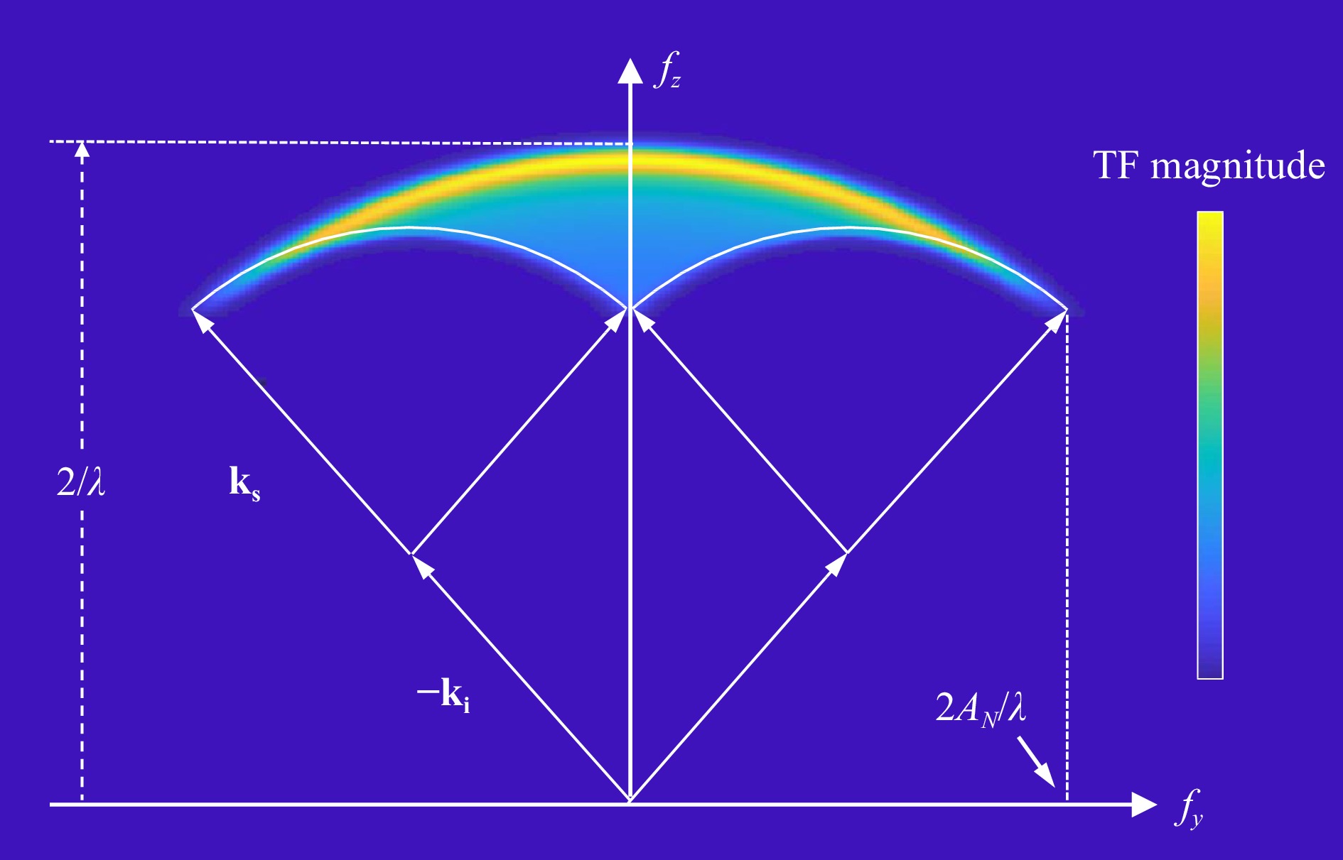

Fig. 23  Geometrical construction of the cross section of a 3D-TF in monochromatic light for an interferometer with a linear pupil filled with incoherent light. The TF magnitude is an arbitrary scale.

As noted by Reynolds, et al., “A hologram is essentially an interferogram, usually made in a division of amplitude interferometer.”¹³² Bryngdahl and Lohmann asserted in 1968 that “…an interferogram is nothing but a special type of a hologram, which we call an ‘image hologram’.”⁸ Going further, Itoh and Ohtsuka proposed that “…it may even be possible to call all the image reconstruction techniques which are based on interferometric measurements of the spatial coherence function as interferometric imaging techniques.”¹³³ With these observations in hand, it can be tempting to conclude that perhaps ‘holography' is just another name for ‘interferometry.’¹³⁴ Fortunately for both fields of study, this is clearly not the case; even if the common principle is the holistic recording and reconstruction of wavefronts using interference patterns.

The birth 60 years ago of practical, laser-based holography resulted in a rapid series of innovations that found their way from holography into interferometry. These advances include using polarization and temporal phase shifting methods, solutions for coherent noise, digital refocusing, interferometric topography measurements of rough surfaces, dynamic interferometry using the off-axis carrier fringe method, and imaging theory using 3D transfer functions. A particularly interesting example is holographic null testing, using computer-generated or experimental holograms. Arguably, the foundations for holographic null testing were laid well over a century ago, for both fabrication and use of diffractive optics for the testing of aspheres and freeforms. But it was not until the discovery of laser-based holography that the technique became a standard for high-precision testing in research and production.

Of course, the selected examples here are far from being a comprehensive list of contributions of holography. One clear trend is the continuously increasing influence of holography on interferometric methods for surface topography measurements. It is possible that this eventually will lead to a fusion of holography with techniques not normally thought of as holographic. This evolution in applied optical metrology will surely lead to significant new solutions going forward.

The authors wish to thank the many contributors to this paper, including Edward LaVilla, who provided the CGH example of Fig. 18, and members of the Zygo Innovations Group, who reviewed the manuscript and participated in excellent discussions regarding the history, meaning and practical use of holographic principles in optics. We offer special thanks to James Wyant, one of the pioneers of holography for interferometric optical testing, for discussions and helpful suggestions.