


-
Holography is a three-dimensional imaging technique. An observer viewing through a hologram can change the depth of focus and the perspective1.
With the advent of digital cameras, Digital Holography became feasible, which had a substantial impact to optical metrology2. Applications range from phase contrast imaging of biological and technical specimen3, volumetric imaging of particle distributions4 and precise shape measurement of functional surfaces5,6. Furthermore, recorded digital holograms of objects or scenes can be directly used as datasets to be displayed by holographic optical displays7,8. The main limiting factor in Digital Holography is the pixel size of the CCD or CMOS device used to record the holograms. The pixel size (distance between the center of neighboring pixels) determines the maximum angle between reference and object wave and thus the recordable object size. This has been widely investigated9,10.
The focus of this article is on the parallax angle under which an object can be reconstructed from a digitally recorded hologram. First holographic reconstructions showing this effect were already published some decades ago11. In this contribution, we will explore the concept of multiple perspective views from the same digital hologram by means of a phase space analysis12,13, which has been proven useful for describing sampling issues and viewing angle specifics in digital holography before14,15. It is well known, that the viewing direction depends on the area of the hologram (i.e. the aperture) through which an observer looks. We will show an easy to comprehend graphical analysis in phase space, which confirms this fundamental property for the case of digital holography as well. Additionally, we will quantitatively investigate how the size and the position of the viewing aperture, and the properties of the camera sensor relate to each other, and which limitations arise from these relations. The result is verified by numerical reconstructions from a digital hologram.
-
The parallax angle
$ \gamma $ is defined in Fig. 1. An object with square-shaped front surface with side length L is located in a distance d from the hologram plane. S is the side length of the recording device. The reference wave is not shown in this figure.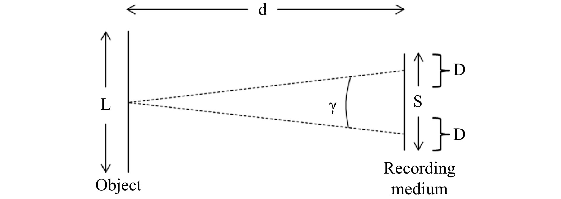
Fig. 1 Definition of the parallax angle
$ \gamma $ (case$ D $ =$ S $ /$ 3 $ is shown).It is not possible to reconstruct a hologram only from a single ray originating from the edge of the hologram. Therefore apertures with finite side length D are defined, which are located at the edges of the recording medium. In Fig. 1 an example with
$ D=S/3 $ is shown. The arms of the parallax angle$ \gamma $ are originating from the centers of the apertures with side length$ D $ , and$ \gamma $ is therefore defined by$$ \begin{align} \gamma \approx \frac{S-D}{d} \end{align} $$ (1) In practice
$ D $ has to be chosen small enough to enable a large parallax angle, but high enough to enable high resolution holographic reconstructions. In classical holography using photographic plates with very fine granularity there are no limitations concerning the plate size, so$ \gamma $ can be increased by enlarging the plate dimensions. In Digital Holography$ S $ has to be replaced by the side length of the image sensor, which is the product of the pixel number N in one direction and the pixel distance$ \Delta p $ :$$ \begin{align} \gamma \approx \frac{N\Delta p-D}{d} \end{align} $$ (2) However, the discrete nature of the camera sensor has important consequences regarding the limitation of the parallax angle. In what follows, we will therefore investigate the dependencies between the pixel pitch
$ \Delta p $ , the recording distance$ d $ , the aperture size$ D $ and the number of pixels$ N $ . This will provide us the means to understand the intrinsic limitations towards the viewing angle$ \gamma $ in Digital Holography when using Eq. 2. Finally, we will also investigate the relationship between the reconstruction quality and the size of the aperture$ D $ and provide experimental validation of the model based on a recorded digital hologram. -
In the following, we will provide a phase space analysis of the concept of viewing directions in Digital Holography. We will not consider the recording process itself, but assume that the complex amplitude
$ u(x) $ of the object wave is determined across the sensor domain, either using off-axis Digital Holography, or inline phase shifting Digital Holography. For more details on the recording process, the reader might wish to refer to Ref. 2.Phase space offers the great benefit of describing the spatial frequency structure of the object wave in arbitrary propagation states. We will make use of the joint space-space frequency representation of the Wigner distribution function (WDF)
$$ \begin{align} W(x, \nu) = \int_{-\infty}^{\infty} u\left( x+\frac{x'}{2} \right) u^{*}\left( x-\frac{x'}{2} \right) \text{exp} \left( - \text{i} 2\pi \nu x'\right) dx' \end{align} $$ (3) Amongst other phase space representations, such as the windowed Fourier transform16, or Gaussian wavelets17, the support of the WDF allows us to assess the impact of apertures and to derive global parameters of the reconstructed wave field based on a simple and concise graphical approach18. We will not revise the mathematical properties of the WDF here. We encourage the interested reader to refer to Bastiaans to study fundamental relations of the WDF in general19, and Testorf and Lohmann for more details on the mathematical properties of the WDF towards Digital Holography20, including various recording configurations.
Instead, we will make use of a common heuristic approach which is based on a graphical representation of the support of the WDF. It treats wave field elements as if they were linearly related to their phase space representation20. In reality this is not the case, because the WDF contains a product relationship which lets arise cross terms. However, in all cases which are discussed in the following, the presence of the cross terms is negligible, because they always lie inside of the considered support of the WDF and therefore do not alter its shape.
-
Phase space depicts space along the
$ x $ -axis and (spatial) frequency along the$ \nu $ -axis. Hence, the corresponding diagrams are two-dimensional even for the case of a one-dimensional wave field. To keep the analysis simple, we will therefore restrict the discussion to the one-dimensional case. However, we will take care, that the extension to two-dimensions is straight forward.Since phase space depicts space and spatial frequencies at the same time, any location
$ x_{0} $ is associated with a corresponding frequency spectrum. In this context, the complex amplitude of a scattered wave field in front of an object can be represented by its support in phase space: Confined along the$ x $ -axis by the size of the object$ L $ and confined along the$ \nu_{x} $ -axis by the maximum propagation frequency$ 1/\lambda $ . This is shown by the grey rectangle in Fig. 2. The area of the rectangle is called the space-bandwidth-product (SBP)18.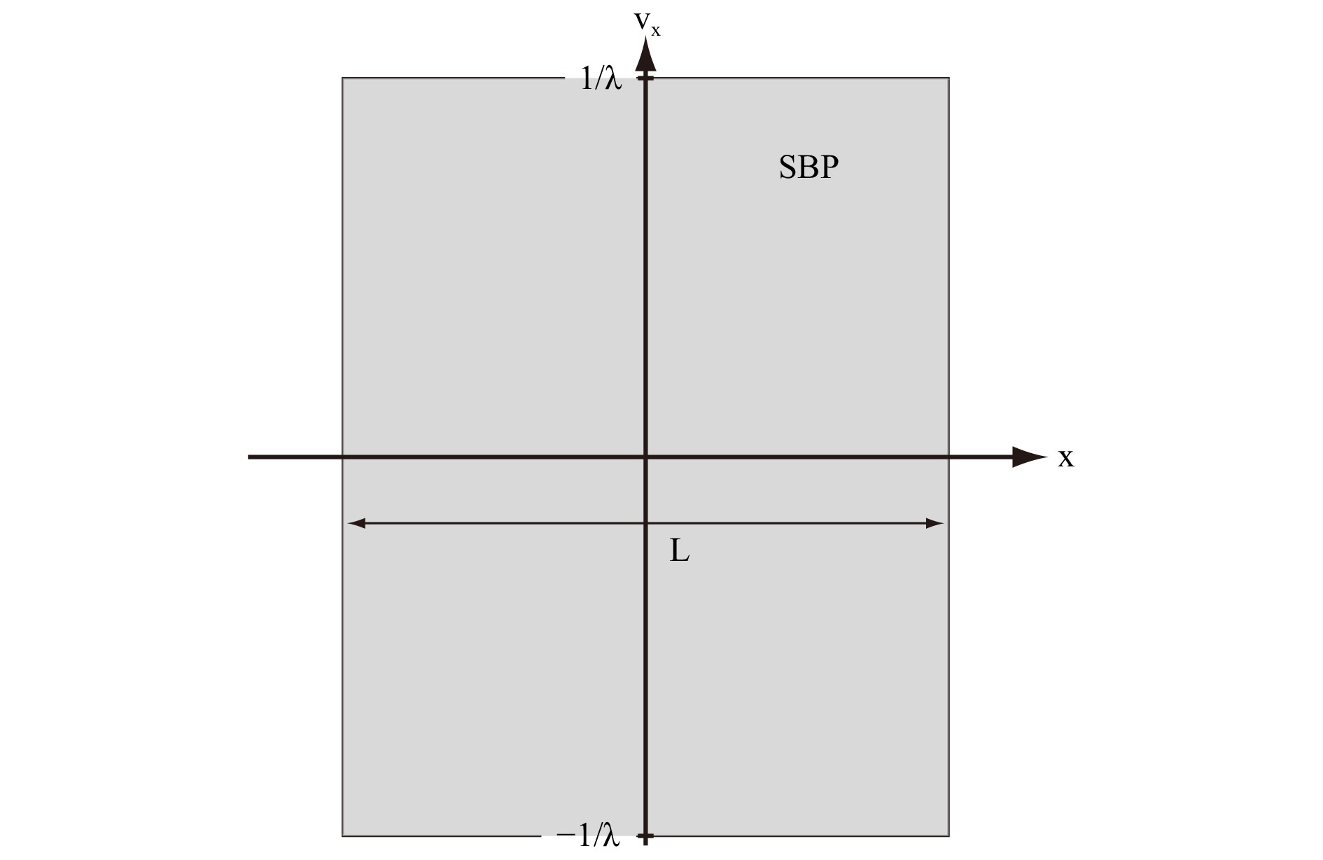
Fig. 2 Support of the complex amplitude of a wave field scattered from an object of size
$ L $ in phase space. For the sake of simplicity, the diagram refers to a$ 1 $ -dimensional wave field. Every spatial position is associated with a spectrum. The area covered by the grey rectangle is called the space-bandwidth-product (SBP).The frequencies
$ \nu_{x} $ can be associated with tilted plane waves and therefore with propagation directions. To visualize this relationship, Fig. 3 depicts a plane wave. Looking at the grey triangle, we recognize that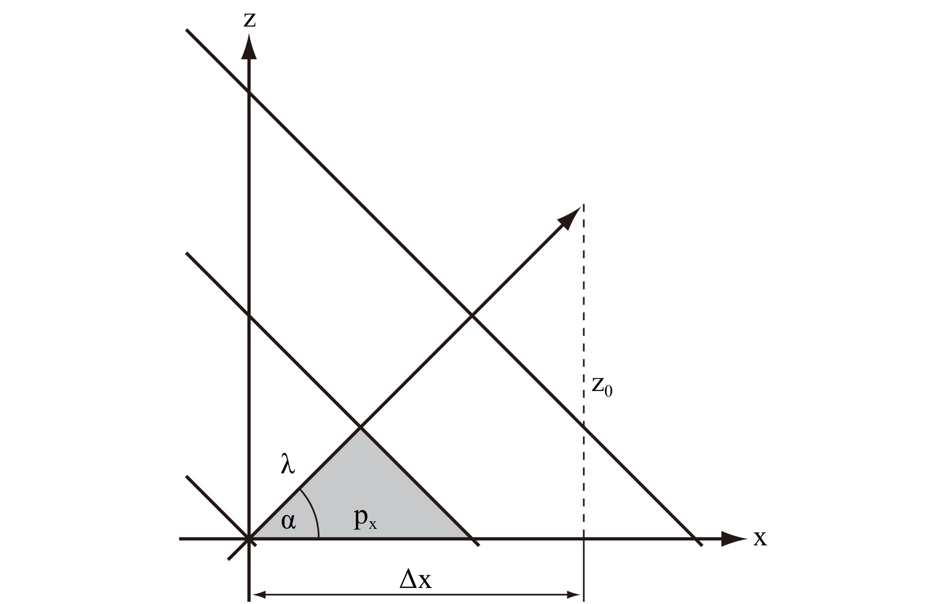
Fig. 3 Propagation of a plane wave: The lines indicate wave fronts. The propagation direction
$ \alpha $ is associated with the spatial frequency$ \nu_{x}=1/p_{x} $ of the complex amplitude in the object plane, as seen from the grey triangle. After propagation of$ z_{0} $ , the wave fronts have also moved laterally by$ \Delta x $ .$$ \begin{align} \cos(\alpha) = \frac{\lambda}{p_{x}} = \nu_{x} \cdot \lambda \end{align} $$ (4) where
$ \alpha $ is the$ x $ -component of the propagation direction with respect to the object plane (not the optical axis!). In case of a two dimensional object plane, we can accordingly define the$ y $ -component of propagation by$ \cos(\beta) = \nu_{y} \cdot \lambda $ , since directional cosines are separable.Fig. 3 is essential to understand how the support of the wave field in phase space changes due to the process of free space propagation. From it, we can infer that any wave field component with frequency
$ \nu_{x} $ will shift in$ x $ -direction while propagating along a given distance$ z_{0} $ . Using Fig. 3 and Eq. 4, it follows:$$ \begin{align} \Delta x(\nu_{x}) = \frac{z_{0}}{\tan(\alpha)} = \frac{z_{0} \cdot \cos(\alpha)}{\sin(\alpha)} \approx \nu_{x} \cdot \lambda \cdot z_{0} \end{align} $$ (5) where we have used the paraxial approximation in the last step, which is justified by the fact that in Digital Holography we almost always deal with waves traveling close to the optical axis, so that
$ \alpha \approx \pi/2 $ and consequently$ \sin(\alpha) \approx 1 $ .As we can see from Eq. 5, under the assumption of paraxial approximation, propagation will cause a shear of the support in phase space, as shown in Fig. 4. The shearing angle can be simply derived from the gradient in Fig. 4, which is given by:
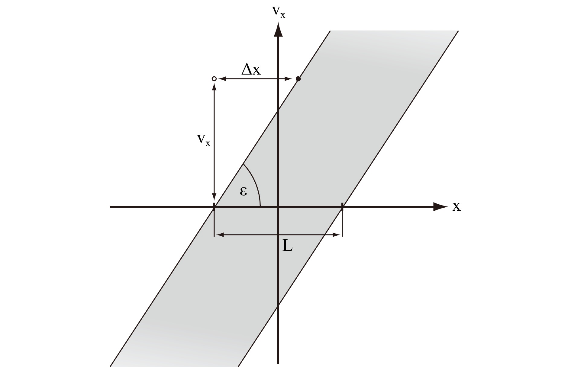
Fig. 4 Propagation in phase space: Since every spectral component also moves laterally during the propagation process, propagation is expressed by a shear of the support. As an example, the spectral component indicated by the disc has been moved from its initial position indicated by the circle by a distance
$ \Delta x $ .$ L $ denotes the spatial extent of the initial wave field in the object plane. From the geometry we can determine the gradient$ \varepsilon $ .$$ \begin{align} \tan(\varepsilon) = \frac{\nu_{x}}{\Delta x} = \frac{\nu_{x}}{\nu_{x} \cdot \lambda \cdot z_{0}} = \frac{1}{\lambda \cdot z_{0}} \end{align} $$ (6) This is all we need to describe the spatial frequency distribution of the object wave during propagation and reconstruction in Digital Holography.
As an example, we can use this scheme to calculate the minimum distance
$ d $ between an object and a camera chip which will ensure the recorded object wave to not contain frequencies above the Nyquist frequency$ \nu_{N}=1/2\Delta p $ . We will assume an object with size$ L $ and a camera chip with size$ S $ and pixel pitch$ \Delta p $ . The situation in phase space is depicted in Fig. 5. From the geometry and Eq. 6 we directly obtain: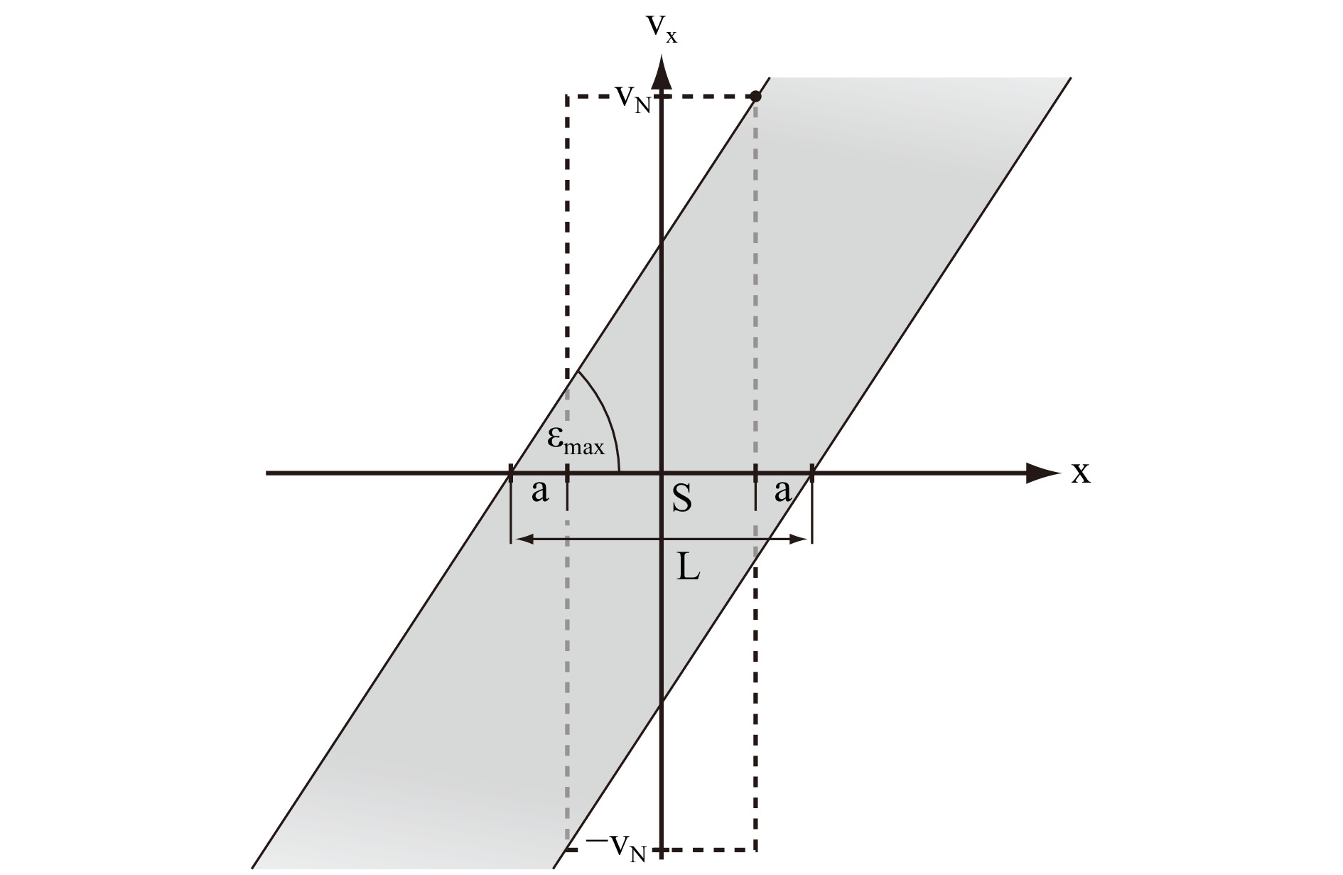
Fig. 5 Minimum propagation distance for Nyquist sampling: The dashed square depicts the SBP of a sensor of size
$ S $ and Nyquist frequency$ \nu_{N} $ . To ensure proper sampling, we have to make sure that the amount of shear is sufficient, so that no frequency incident on the sensor exceeds the Nyquist frequency. Evaluating the corresponding maximum gradient$ \varepsilon_{max} $ allows to determine the minimum propagation distance. Please, refer to the text for details.$$ \begin{align} \tan(\varepsilon_{max})=\frac{\nu_N}{a+S}=\frac{1}{\lambda d} \end{align} $$ (7) Rearranging the equation and using the pixel distance
$ \Delta p $ rather than the Nyquist frequency yields$$ \begin{align} d=\frac{2\Delta p}{\lambda}(a + S) \end{align} $$ (8) From Fig. 5 we see that
$ a=(L-S)/2 $ . If we further assume$ S=N \cdot \Delta p $ , with$ N $ the number of pixels in one direction of the sensor, we finally arrive at$$ \begin{align} d = \frac{\Delta p}{\lambda}(L+N\Delta p) \end{align} $$ (9) Since spatial frequencies are separable in the frequency domain, the extension to two dimensions is again straight forward. In this case,
$ L $ would rather represent the largest extent$ L_{x} $ of the object in$ x $ -direction. Accordingly we can define$ L_{y} $ as the largest extent in$ y $ -direction. In order to ensure Nyquist sampling in this case, the larger value has to be inserted as$ L $ into Eq. 9 (assuming a square sensor with equal pixel number$ N $ and pixel pitch$ \Delta p $ in both directions). However, please note that even if it is convenient, it is not mandatory to adhere to the Nyquist sampling in Digital Holography, because the specific structure of the propagated object wave in phase space allows the application of generalized sampling approaches21. -
Up to now, we have not identified any viewing directions. The wave field originating from a digital hologram does not provide any viewing directions per se, since light is simply propagating in all directions at the same time. The concept of a specific viewing direction therefore always involves the choice of a limiting aperture. Consequently, to generate a viewing direction, we have to insert a digital aperture and set all parts of the hologram outside of this aperture to zero. This will have two important consequences for the reconstruction process. Firstly, we only reconstruct parts of the wave field that traveled along the direction defined by the aperture. This is what gives us the impression of looking at the object or scene from a specific direction. Secondly, the resolution of the reconstruction will be reduced according to the size of the aperture in the hologram plane.
As shown in Fig. 6, we can quantify both effects in phase space. Fig. 6a depicts the object wave in phase space across the area given by the SBP of the camera sensor and Fig. 6b after propagation into the object plane. As an example, we have chosen to define two digital apertures of size
$ D=S/2 $ , indicated by the letters$ A $ and$ B $ , which will provide us with view$ A $ and view$ B $ on the object. The average viewing directions can be simply derived by finding the centers of the apertures. The corresponding frequencies$ \nu_{A} $ and$ \nu_{B} $ define the viewing directions in accordance with Eq. 4. From Fig. 6a and Eq. 6 we find for example for view$ A $ 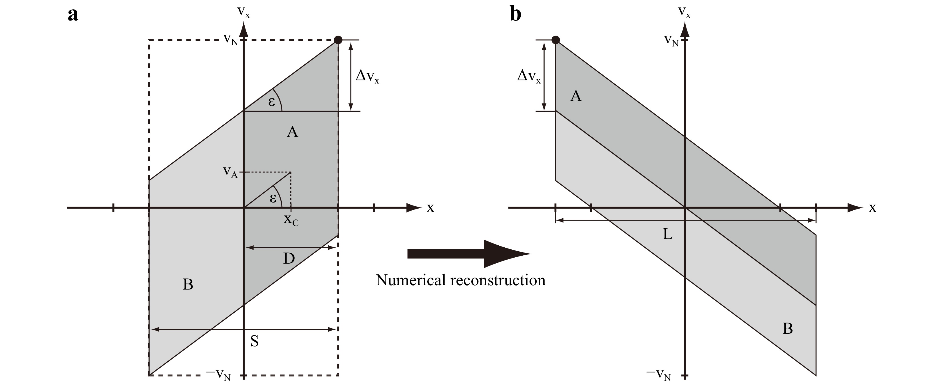
Fig. 6 a The support of the propagated object wave is divided into two views indicated by the different grey values and the letters
$ A $ and$ B $ . Experimentally, this can be realized by a digital aperture, which sets all values of the complex amplitude outside of the aperture to zero. In this example the apertures that provide the views$ A $ and$ B $ have the size$ D $ and are centered around$ x_{C} $ and$ -x_{C} $ .$ S $ indicates the size of the sensor. b The support in phase space after numerical reconstruction of the object wave into the object plane.$ \Delta \nu_{x} $ indicates the local bandwidth of the wave field, which can be used to determine the resolution, and$ L $ is the size of the object. For more details, please refer to the text.$$ \begin{align} \tan(\varepsilon) = \frac{\nu_{A}}{x_{C}} = \frac{1}{\lambda \cdot z_{0}} \end{align} $$ (10) where
$ x_{C} $ denotes the center of the aperture. Inserting this into Eq. 4 with$ \nu_{x}=\nu_{A} $ yields$$ \begin{align} \cos(\alpha_{A}) = \nu_{A} \cdot \lambda = \frac{x_{C}}{z_{0}} \end{align} $$ (11) The viewing direction
$ \alpha_{A} $ so found is defined with respect to the hologram plane. If we want to define it more conveniently with respect to the optical axis, we use$ \zeta = \pi/2 - \alpha_{A} $ and find for small angles$ \zeta $ $$ \begin{align} \cos(\alpha_{A}) = \sin(\zeta) \approx \zeta = \frac{x_{C}}{z_{0}} \end{align} $$ (12) View
$ A $ and view$ B $ are only the limiting cases for a hologram with size$ S $ . In principle, we can select any digital aperture with size$ D $ between the positions$ -x_{C} $ and$ x_{C} $ , which gives us the total viewing range of$ 2\zeta $ . Indeed, if we insert$ x_{C}=(S-D)/2 $ and$ z_{0}=d $ , we can compare Eq. 12 with Eq. 1 to verify$ \gamma = 2\zeta $ .It is important to note, that because of the definition of
$ \zeta $ towards the optical axis, Eq. 12 cannot be straight forward extended to$ 2 $ dimensions. Instead we will assume, that in the two dimensional case, the aperture is only limiting in$ x $ -direction, i.e. the hologram is separated into a left view$ A $ and a right view$ B $ , so that$ \zeta $ lies in the$ x $ -$ z $ -plane, in analogy to the scheme introduced by Fig. 1.Assuming that no other optical elements, e.g. lenses, are used, it is clear from Fig. 6a that there are only two possible ways to increase the viewing range: Firstly we could reduce the pixel pitch
$ \Delta p $ , which would increase the Nyquist frequency$ \nu_{N} $ , and secondly we could enlarge$ x_{C}=(S-D)/2 $ by reducing the size of the aperture$ D $ . The latter, however, will further decrease the resolution of the reconstructed object wave, as we will see below.Let us now insert Eq. 9 into Eq. 2, in order to quantitatively assess the limitations arising from the discrete recording device:
$$ \begin{align} \gamma = \frac{N\lambda}{(L+N\Delta p)} \left(1 - \frac{D}{N \Delta p} \right) \end{align} $$ (13) The side length of the aperture
$ D $ will always be a fraction$ \kappa $ of the side length of the sensor$ S $ , so that$ D=\kappa S = \kappa N \Delta p $ with$ \kappa \leq 0.5 $ . This means, that the last term in Eq. 13 is a constant, and we finally yield$$ \begin{align} \gamma = \frac{N\lambda}{(L+N\Delta p)} (1 - \kappa) \end{align} $$ (14) From Eq. 14, we see that the parallax angle
$ \gamma $ solely depends on the object size L and on the pixel size of the sensor$ \Delta p $ if N and$ \lambda $ are fixed. This is shown graphically in Fig. 7, where$ \gamma $ is plotted on the y-axis and$ \Delta p $ is plotted on the x-axis. Four curves are shown with$ N=1000 $ ,$ N=2000 $ ,$ N=3000 $ and$ N=4000 $ . For all$ 4 $ curves$ L= 1 $ cm,$ \lambda=633 $ nm and$ \kappa=0.5 $ are chosen. It can be seen in all four curves that the parallax angle increases with decreasing pixel size. That means image sensors with small pixel sizes of about 1$ \mu $ $ m $ are advantageous to allow larger changes of perspective in Digital Holography. Today available CMOS sensors have pixel sizes down to 1,6$ \mu $ $ m $ and more than$ 10 $ million pixels, enabling parallax angles of several degrees.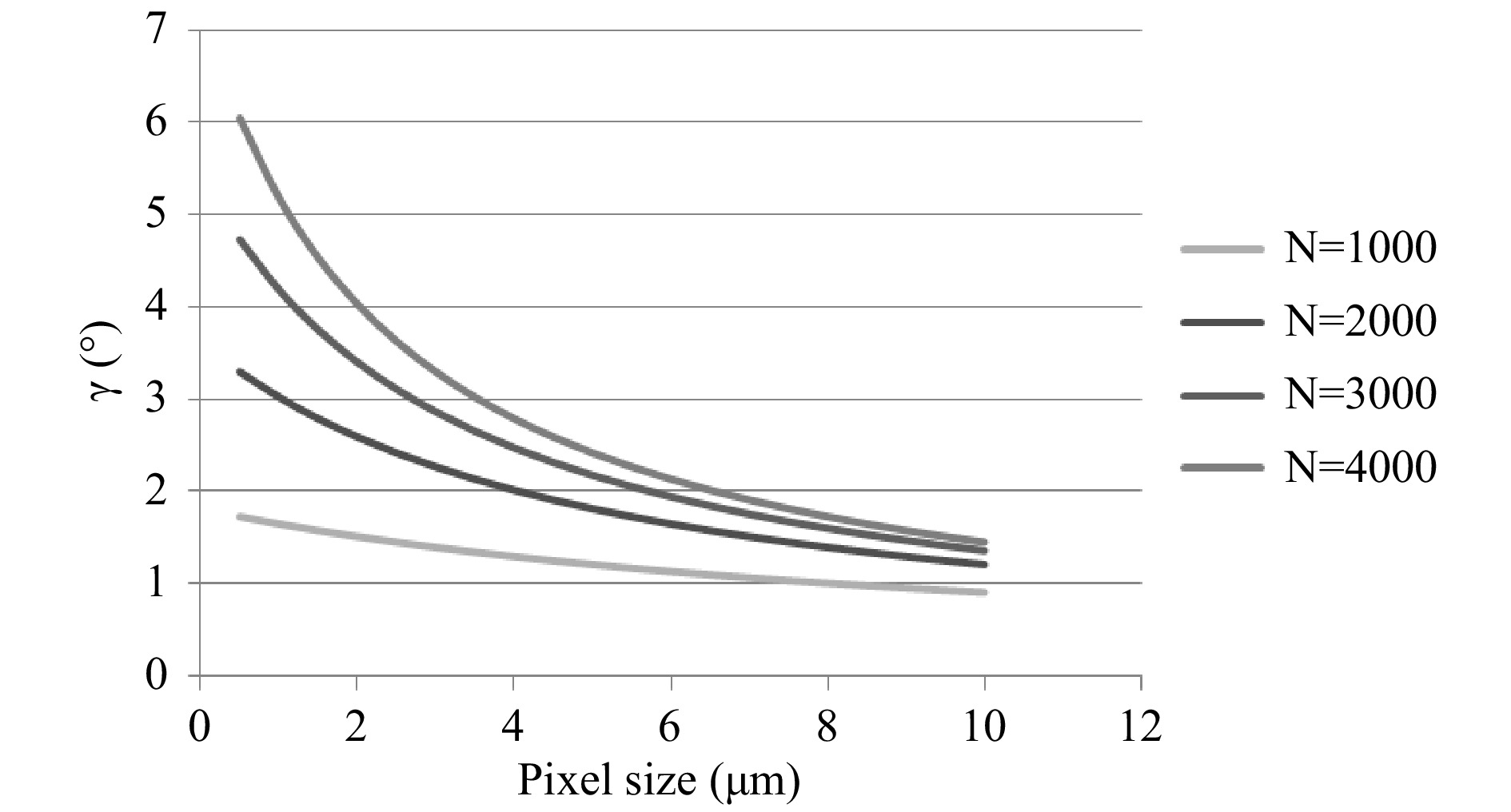
Fig. 7 Parallax angle in degrees (y-axis) versus pixel size in micron (x-axis) for different pixel numbers
In addition it can be concluded by comparison of the curves, that increasing the number of pixels
$ N $ does not lead to a significantly larger parallax angle for large pixel sizes around$ 10 $ $ \mu $ $ m $ . Significantly larger angles can be achieved by enlarging$ N $ only with small pixel sizes of approx. 1$ \mu $ $ m $ . This effect becomes clearer if we focus on small objects ($ L<<N\Delta\,p $ ). In this case, Eq. 14 can be further approximated:$$ \begin{align} \gamma=\frac{\lambda}{\Delta p}(1-\kappa) \end{align} $$ (15) Now
$ \gamma $ is inversely proportional to$ \Delta p $ and independent from the pixel number N. An increase of$ N $ has no effect on$ \gamma $ because the necessary larger distance between object and sensor compensates the effect of the higher pixel number. Methods proposed earlier to enlarge the aperture by using several image sensors in parallel22 are therefore not suitable to increase the parallax angle. -
We can assess the resolution of the reconstructed object wave, when we perform the numerical reconstruction. In phase space, this means we invert the shearing process of the support as shown in Fig. 6b. Again view
$ A $ and view$ B $ are indicated. As we can see, due to the limited SBP of the aperture, the bandwidth of the reconstructed object wave is significantly reduced. Even though the support of each view covers a large area in frequency space, the resolution is solely defined by the local bandwidth$ \Delta \nu_{x} $ . In fact, the inclined structure of the support indicates a wave front chirp, which does not carry any information. Comparing Fig. 6b with Fig. 6a, we see from the geometry, that$$ \begin{align} \Delta \nu_{x} = D \cdot \tan(\varepsilon) = D \cdot \frac{1}{\lambda \cdot z_{0}} \end{align} $$ (16) holds. If we consider the numerical aperture of the aperture
$ NA_{D}=D/2z_{0} $ and the minimum detail to be resolved as the inverse of the bandwidth$ d_{x} = 1/\Delta \nu_{x} $ , Eq. 16 turns into the well known diffraction limited resolution for a rectangular aperture$$ \begin{align} d_{x} = \frac{\lambda}{2\cdot NA_{D}} \end{align} $$ (17) Since we assumed the digital apertures to be only limiting in
$ x $ -direction, the point-spread-function of the reconstructed object wave will be elongated in this direction. In$ y $ -direction we will need to insert the numerical aperture of the sensor chip$ NA_{S}=S/2z_{0} $ into Eq. 17 to obtain$ d_{y} $ . -
Phase shifting Digital Holography is used to demonstrate the change of perspective if different parts of a hologram are used for reconstruction. A CMOS sensor with
$ 2054 \;\times \; 2452 $ pixel and a pixel pitch of$ 3.45 $ $ \mu $ m$ \times $ $ 3.45 $ $ \mu $ m is used. The wavelength is$ 532 $ nm. The object is placed in a distance of$ 0.175 $ m from the sensor. The effective width of the brick used as object in viewing direction is$ L \approx\ 1.7 $ cm. A plane reference wave and the object wave interfere on the surface of the sensor. The initial phase in the hologram plane is recorded using phase-shifting. The numerical reconstruction into the object area is done with the Fresnel approximation. The resulting image resolution (pixel distance in the reconstructed image) is$ 11.0 $ $ \mu $ m$ \times $ $ 13.1 $ $ \mu $ m. These values are not equal due to the different pixel numbers in x- and y-direction. A reconstruction using the entire hologram matrix ($ 2054\; \times\; 2452 $ pixel) is shown in Fig. 8.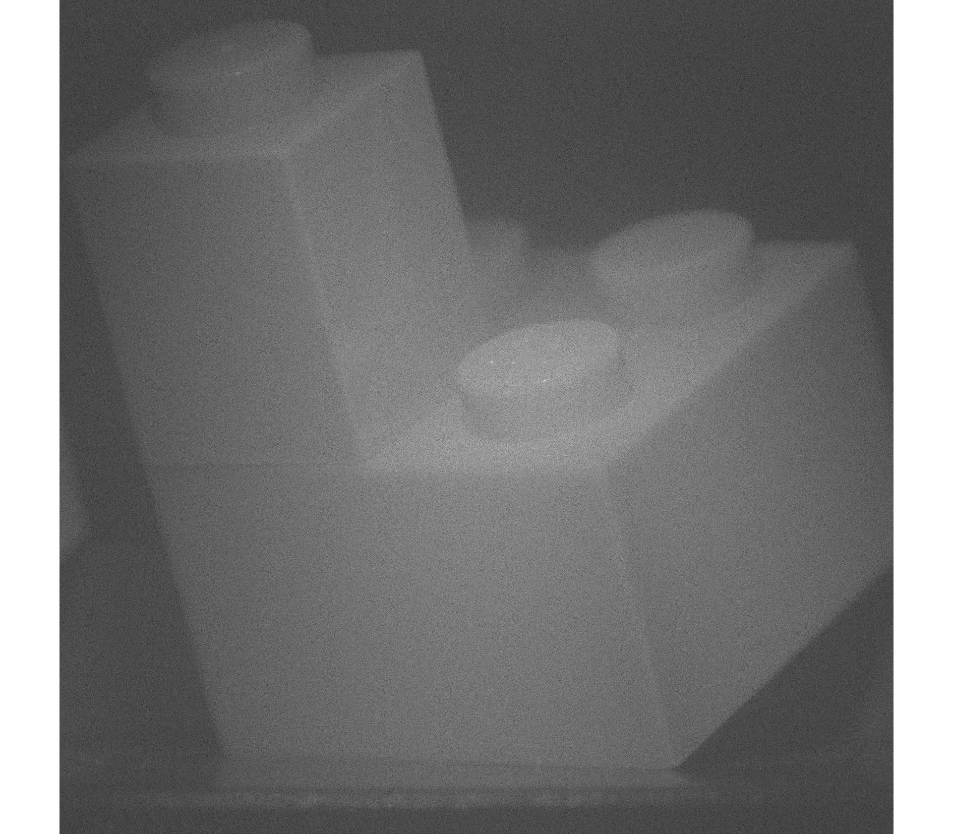
Fig. 8 Reconstruction of a hologram using the entire hologram matrix (2054 × 2452 pixel, image rescaled to quadratic shape).
Views from different angles are generated by two reconstructions with only
$ 2054\; \times\; 800 $ pixel ($ \kappa=0.33 $ ). A view from the left is generated by using only the columns$ 1 $ to$ 800 $ of the hologram matrix, the grey values of the other columns are set to zero (zero padding). This reconstruction is shown in Fig. 9. A view from the right is generated by using only columns$ 1652 $ to$ 2452 $ ; the grey values of the other pixel are set to zero. This view is shown in Fig. 10. The speckle size in both images, Fig. 9 and Fig. 10, is larger than in Fig. 8. This is due to the smaller aperture (lower number of pixel in horizontal direction) used for the reconstructions.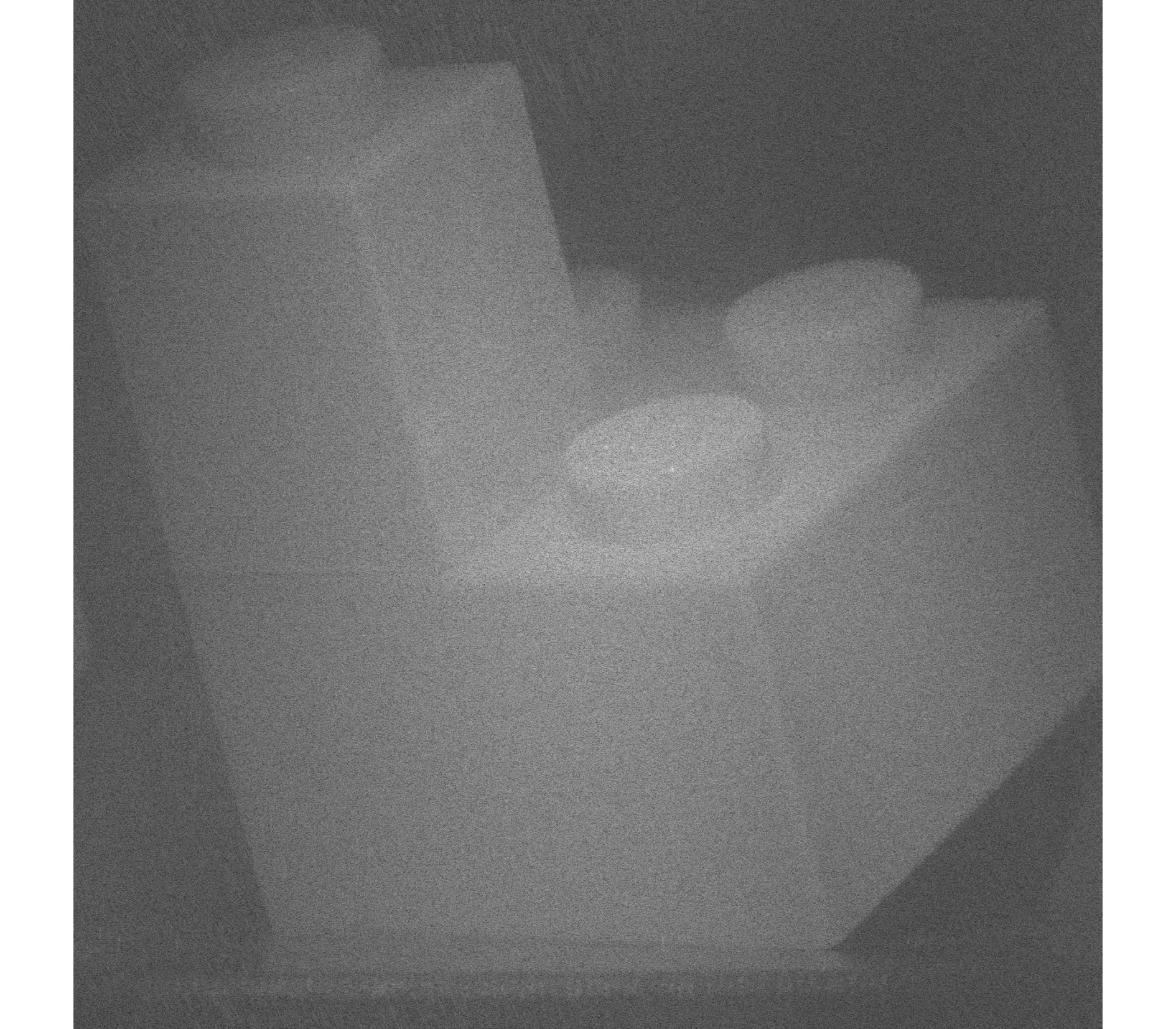
Fig. 9 Reconstruction from the left stripe of the hologram matrix (2054 × 800 pixel).
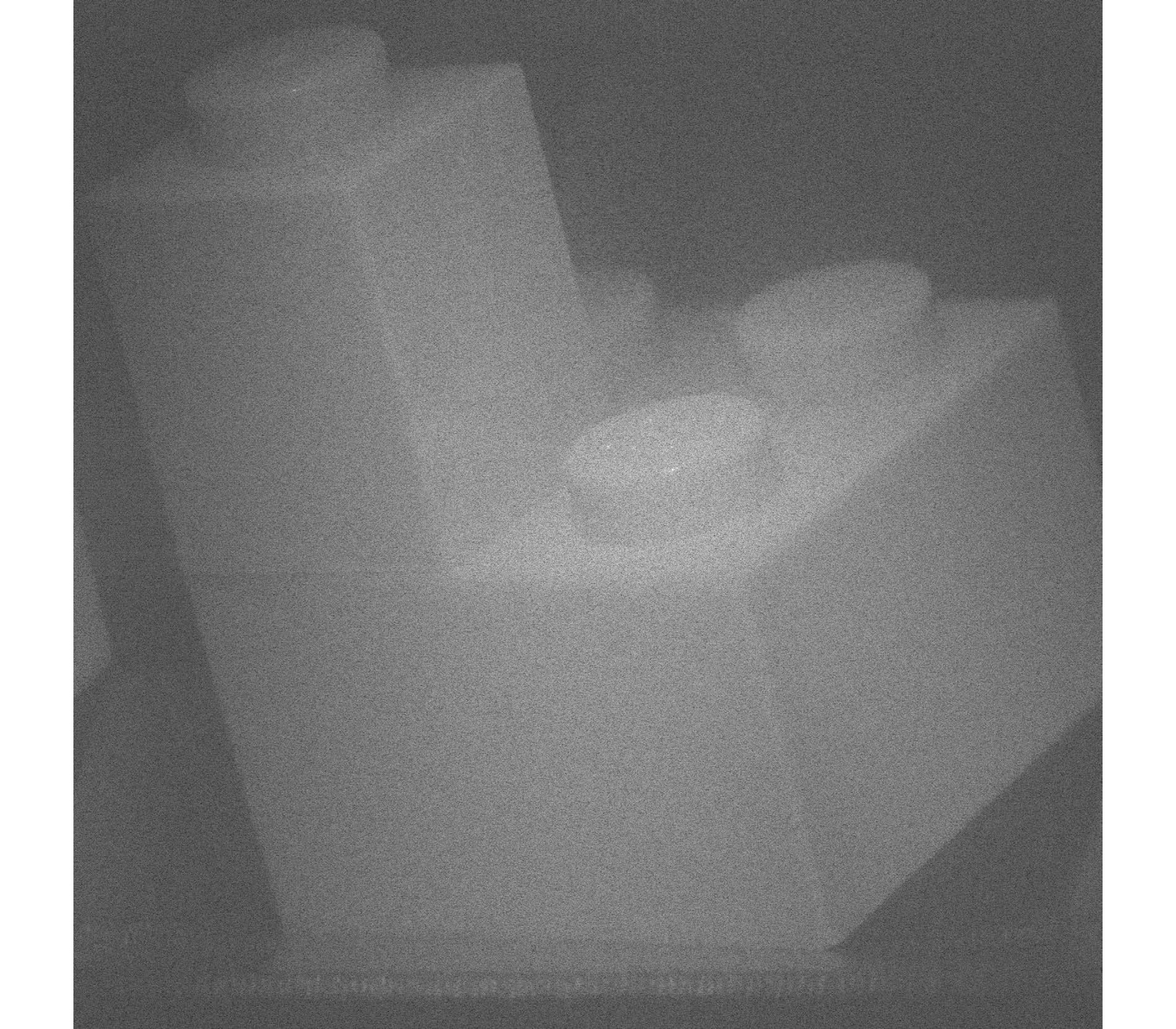
Fig. 10 Reconstruction from the right stripe of the hologram matrix (2054 × 800 pixel).
The change of perspective is small but visible by comparing Fig. 9 and Fig. 10. The viewing direction on the knobs on top of the lower brick is slightly different. The real parallax angle according to Eq. 2 is
$ \gamma = 1.85^{\circ} $ . This is only slightly lower than the theoretical maximum angle calculated with Eq. 14 of$ \gamma_{th} = 1.96^{\circ} $ degrees. The perspective change is visible more clearly in the video provided as supplementary material. -
Parallax in Digital Holography has been analyzed using a phase space approach. It has been shown that the parallax angle depends on the pixel size of the image sensor. The smaller the pixel size the larger is the parallax angle. Increasing the pixel number leads to a noticeable increase of the parallax angle only for sensors with small pixel sizes. An experimental example shows that different views can be reconstructed from a single hologram. The predicted change of perspective is small, but visible in Digital Holography. The phase space approach is an appropriate tool to calculate parallax angles in Digital Holography. With state of the art CCD or CMOS devices the viewing angle change is very small. However, future devices might have pixel sizes below one micron. Large parallax changes comparable to those of classical film holography will be possible, enabling new applications in imaging.
-
The holographic set-up consists of a Michelson-type interferometer. A plane wave is split at the beam splitter into two partial waves. The reference wave is guided to a mirror in one arm of the interferometer. The other wave illuminates the object and is reflected from there. The plane reference wave and the diffusely reflected object wave are recombined at the beam splitter and interfere at the surface of the CMOS sensor. The initial phase of the wave in the sensor area is generated with the help of a phase shifting unit.
Numerical reconstruction of the wave into the object area is done with the Fresnel approximation. The code is implemented in MATLAB.
More details of the recording process and of the numerical reconstruction are described in the literature, the reader is referred to Ref. 2.
-
We would like to thank Prof. Ralf B. Bergmann for fruitful discussions. The experimental results presented here are based on digital holograms recorded in the laboratories of BIAS - Bremer Institut für angewandte Strahltechnik GmbH. We are grateful to Thomas Meeser for experimental support with the hologram recordings. The recordings were performed within the frame of project 'Real 3D', funded by the EU 7th Framework Program FP7/2007-2013 under agreement 216105.
Parallax limitations in digital holography: a phase space approach
- Light: Advanced Manufacturing 3, Article number: 28 (2022)
- Received: 26 August 2021
- Revised: 05 April 2022
- Accepted: 20 April 2022 Published online: 20 June 2022
doi: https://doi.org/10.37188/lam.2022.028
Abstract: The viewing direction in Digital Holography can be varied if different parts of a hologram are reconstructed. In this article parallax limitations are discussed using the phase space formalism. An equation for the parallax angle is derived with this formalism from simple geometric quantities. The result is discussed in terms of pixel size and pixel number of the image sensor. Change of perspective is demonstrated experimentally by two numerical hologram reconstructions from different parts of one single digital hologram.
Research Summary
Digital Holography: Parallax Limitations calculated with a Phase Space Approach
The viewing direction in Digital Holography can be varied if different parts of a hologram are reconstructed. In this article parallax limitations are discussed using the phase space formalism. An equation for the parallax angle is derived with this formalism from simple geometric quantities. The result is discussed in terms of pixel size and pixel number of the image sensor. Change of perspective is demonstrated experimentally by two numerical hologram reconstructions from different parts of one single digital hologram.


Rights and permissions
Open Access This article is licensed under a Creative Commons Attribution 4.0 International License, which permits use, sharing, adaptation, distribution and reproduction in any medium or format, as long as you give appropriate credit to the original author(s) and the source, provide a link to the Creative Commons license, and indicate if changes were made. The images or other third party material in this article are included in the article′s Creative Commons license, unless indicated otherwise in a credit line to the material. If material is not included in the article′s Creative Commons license and your intended use is not permitted by statutory regulation or exceeds the permitted use, you will need to obtain permission directly from the copyright holder. To view a copy of this license, visit http://creativecommons.org/licenses/by/4.0/.

 DownLoad: