


-
Minimally invasive in vivo imaging at hardly accessible locations is crucial for many biomedical applications inside the human body, such as calcium imaging1. Moreover, there is a great research interest in supervising structural and functional processes like brain activity in freely moving animals at cellular resolution2, 3. While the observation of neuronal activity in living animals was demonstrated with two-photon microscopy up to a depth of 550 µm4, imaging deeper inside the brain requires flexible, minimally invasive endoscopes. Therefore, in vivo endoscopic imaging systems need to be robust towards bending and ultra-thin to reduce damage to cells and tissue. Furthermore, three-dimensional (3D) imaging capabilities including high spatial and temporal resolution, chromatic sensitivity and large field of view (FoV) are desired5.
State-of-the-art lens-based coherent fiber bundle (CFB) endoscopes only allow two-dimensional (2D) imaging in the focal plane of the lens. The CFB enables pixelwise intensity transfer, thus limiting the space-bandwidth product (SBP) by the core number. Therefore, the resolution is determined by the fiber core pitch and the magnification. The use of microlenses allows trading off lateral for axial resolution6, 7. Focus tunable lenses and piezo actuators exchange axial for temporal resolution, but are only available at diameters far above 1 mm8, 9. 3D imaging can be achieved by using stereo probes, however, the added constructive complexity can be hard to miniaturize effectively10. The smallest endoscope diameters can be achieved with single-mode fibers. In combination with Optical Coherence Tomography, 3D imaging of mouse veins was achieved at probe diameters below 0.5 mm11. However, coherent light is needed, which prevents applications like fluorescence imaging, and a mechanical focus scanning movement is necessary, which increases the complexity of the sensor head12. Multimode fibers (MMF)13−19 as well as coherent fiber bundles (CFB)20−26 enable lensless endoscopic imaging with passive probe tips and diameters below 500 µm. A high SBP and 3D object reconstruction can be achieved via holography27−31 or time-of-flight approaches32. However, as the aforementioned lensless endoscopy approaches rely on phase reconstruction, they are prone to fiber bending and require coherent light. The necessary in situ phase recalibration limits the temporal resolution and the measurement of incoherent fluorescent light is challenging. This restricts the transfer to real-world applications.
The use of a CFB and a coded aperture is promising for both 3D imaging with incoherent illumination33 as well as a higher SBP than equivalent lens-based endoscopes in 2D-imaging scenarios34, 35. The light and information loss of coded apertures can be evaded by using diffuse phase masks36−38. In any case, computational image reconstruction is necessary. There are multiple iterative approaches for object retrieval based on convex optimization39, 40, but they do not offer suitable reconstruction speeds for in vivo real-time imaging. In contrast, neural networks41−45 enable operation at video rate after completing the training process46, 47 and 3D48 image reconstruction. Moreover, they are robust towards model errors and do not rely on point spread function (PSF) shift invariance49.
In this paper, we demonstrate a minimally invasive diffuser-based fiber endoscope with single-shot 3D live fluorescence imaging capabilities and a probe tip diameter of 700 µm, allowing minimally invasive applications for instance in neurosurgery. The setup is shown in Fig. 1a. Laser light illuminates the tissue through the fiber endoscope. Incoherent light emitted by fluorescent 3D objects is encoded by the diffuser into 2D speckle patterns. The speckle patterns are transmitted by the CFB onto a camera. The 3D object is then computationally reconstructed by neural networks in 20 ms, allowing video-rate imaging at up to 50 fps. Because our approach only processes intensity images, dispersion between fiber cores from optical path length differences as well as phase shifts due to bending can be ignored34. In fluorescence settings, the setup can be used for illumination and detection simultaneously, enabling biomedical applications for in vivo imaging at cellular resolution like calcium imaging (Fig. 1b).
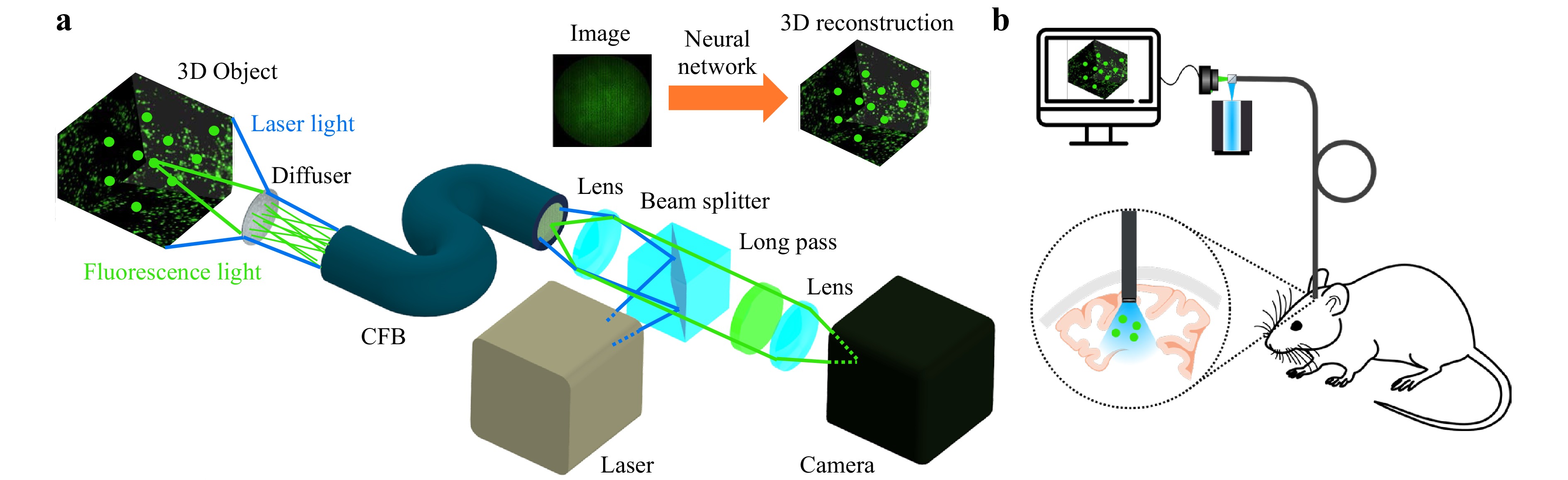
Fig. 1 a Fluorescence Imaging Setup. A fluorescent object (2D/3D) is illuminated through the system by a laser. Incoherent light emitted by the object is encoded into 2D speckle patterns by a diffuser. The intensity pattern is transmitted by a coherent fiber bundle (CFB) onto a camera. The object image is then computationally reconstructed by a neural network. b Potential application of the diffuser endoscope for in vivo calcium imaging to observe deep brain activity in living animals.
-
To investigate the suitability of the diffuser endoscope for 2D and 3D imaging, different simulation and laboratory experiments were conducted. The approach was first tested in silico in a 2D modality. The system was simulated using Fourier optics to generate pairs of ground truth and camera images as a training dataset. We found a neural network architecture consisting of a combination of Single Layer Perceptron (SLP) and U-Net offered the best reconstruction quality and generalization capabilities. More details on the simulation as well as the neural network training and reconstruction can be found in the Materials and Methods chapter. The reconstruction quality of this and the following experiments was assessed with the metrics of peak signal-to-noise ratio (PSNR), structural similarity index measure (SSIM) and correlation coefficient (CC) in Table 1. For the 2D simulation in a FoV of 416 µm × 416 µm at a distance z of 700 µm between the object plane and the diffuser (Fig. 2a), the evaluation metrics including a mean SSIM of 0.91 indicate a reconstruction with great fidelity.
Metric 2D Sim
(n = 1000)2D Exp
(n = 4)3D Sim
(n = 1000)3D Exp
(n = 4)PSNR 28.4 dB 25.3 dB 30.5 dB 29.5 dB SSIM 0.91 0.89 0.92 0.82 CC 0.93 0.84 0.72 0.43 Table 1. Mean reconstruction quality for the simulation and lab experiments
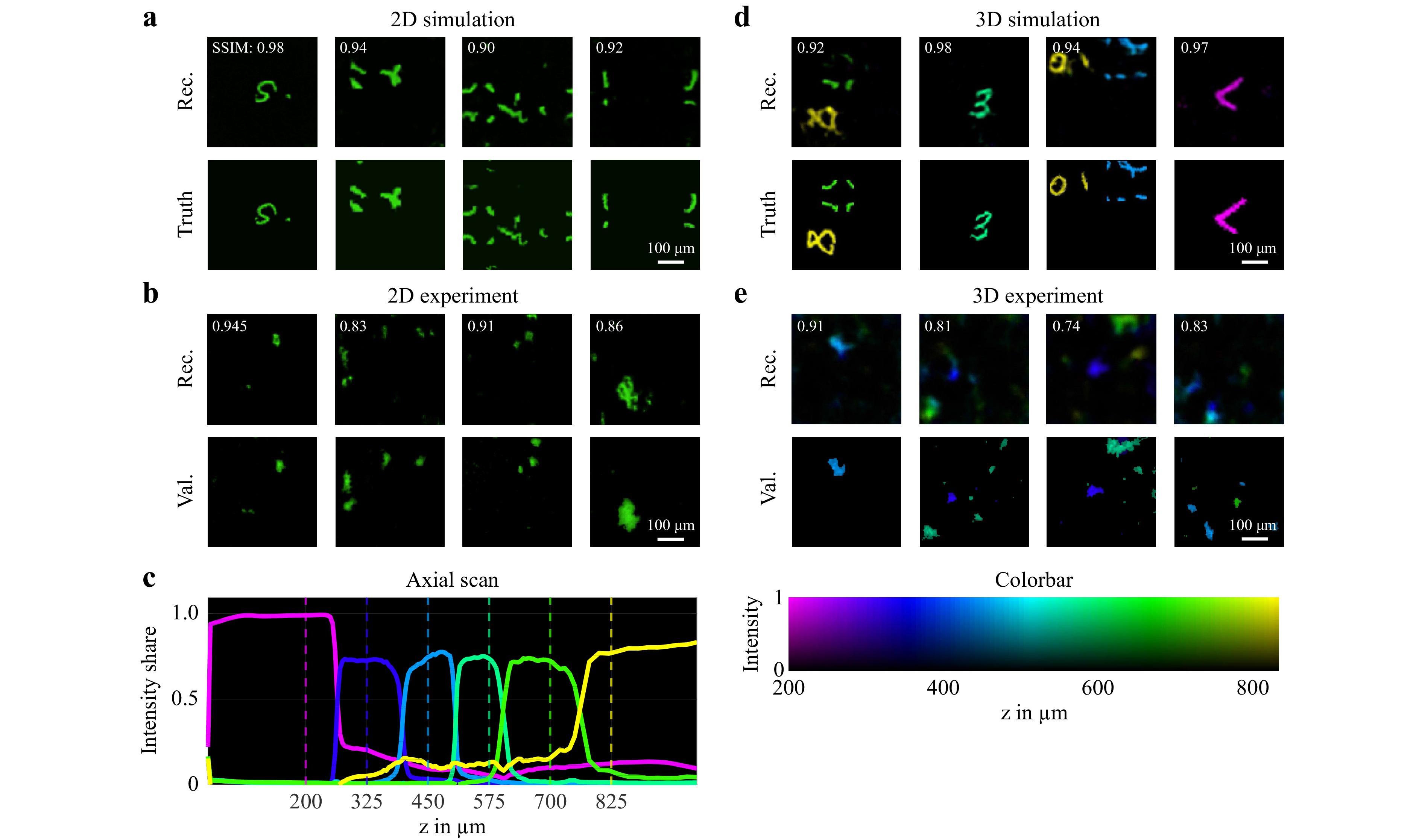
Fig. 2 a 2D reconstruction of simulated system trained with augmented MNIST digit data. (top) Neural network reconstruction (2D). (bottom) Ground truth images (2D). b 2D imaging experiment with fluorescence particles at a distance of z = 800 µm from the diffuser. (top) 2D image reconstruction by neural network. (bottom) 2D ground truth captured by validation microscope. c Intensity share of reconstruction plane for axial scan of projected square over z. The dashed lines mark the positions of the depth planes used for the neural network training. d 3D reconstruction of simulated system trained with augmented MNIST digit 3D data. The depth position of each voxel in the 3D images is displayed by the color according to the colorbar on the right. (top) Neural network reconstruction (3D). (bottom) Ground truth images (3D). e 3D imaging experiment with fluorescence particles at two distances z between 200 µm and 800 µm from the diffuser. (top) 3D image reconstruction by neural network. (middle) 2D ground truth for z = 400 µm captured by validation microscope. (bottom) 2D ground truth for z = 575 µm captured by validation microscope. The depth position of each voxel in the 3D images is displayed by the color according to the colorbar on the bottom.
Next, the 3D imaging capability was validated. Therefore, the simulation and the neural network architecture was extended to a FoV of 416 µm × 416 µm × 625 µm consisting of six equally spaced depth layers. Example reconstructions are shown in Fig. 2d where the depth position of each voxel is displayed by a color according to the colorbar on the bottom right. This simulation experiment demonstrates the 3D imaging capabilities of the system. However, the mean PSNR and SSIM values are deceptively high, because the 3D objects are sparsely occupied.
For the validation of these simulation experiments, a setup for imaging of fluorescent Rhodamine B particles was used (Fig. 1a). A digital light projector was employed to project images from six equally spaced axial distances between 200 and 825 µm into the system to train reconstruction networks with a 3D output. The setup and signal processing was then tested by imaging fluorescent particles in 2D and 3D, that were illuminated from the proximal side through the CFB. In both cases, we were able to show that the generalization ability of the networks was sufficient to locate few particles in the FoV. However, the reconstruction quality is reduced with decreasing object sparsity. The reconstruction quality for the fluorescence experiments is worse than it was for the simulations, which could result from the unoptimized diffuser endoscope setup, noise and the difficult generalization task for the networks.
To validate the depth perception, an object was projected in front of the endoscope at varying axial positions and reconstructed by the neural network. In Fig. 2c, the intensity shares of the reconstructed outputs at the six depths are shown over the projection distance z. With at least 70% of the intensity attributed to the correct depth plane, an unambiguous discrimination between the axial positions is achieved. Given by the distance between the trained depth planes, an axial resolution of 125 µm results. From the steepness of the slopes in Fig. 2c it follows, that this can be improved further up to 10 µm, e.g. by adding more depth layers to the network architecture, see section ‘Materials and methods - Field of view and resolution’.
For both cases of single-shot 2D and 3D imaging, the neural networks are able to reconstruct the image in under 20 ms. The exposure time of around 100 ms was limited by the illumination power of 5 mW in the probe volume, resulting in a total frame rate of 8 fps. No image averaging was performed. Depending on the permitted phototoxicity levels50, the illumination power and therefore the frame rate can be further increased.
-
The diffuser fiber endoscope we present in this paper was used to demonstrate single-shot 2D and 3D fluorescence imaging with proximal illumination through the CFB, potentially enabling applications like calcium imaging, cancer diagnostics or 3D flow measurement. While this system offers many advantages in comparison to similar approaches, there are also certain limitations that need to be considered.
For many clinical applications, the robustness of the imaging system is an important requirement. In contrast to holographic approaches, no coherent light is required for fluorescence imaging. By using incoherent illumination, only the intensity carries useful information while the phase can be omitted. This makes the imaging system robust towards bending of the fiber bundle which benefits all in vivo applications. Furthermore, the endoscope length should not be a limiting factor for biomedical applications, as long as the signal-to-noise ratio is high enough. The system was illuminated with a laser for the presented experiments, which could be replaced by an LED. This could prevent illumination speckles. Moreover, the diffuser-based endoscope can offer a higher space-bandwidth product than an equivalent lens-based endoscope (Fig. 5), which could also be useful whenever a bigger FoV could make the orientation easier and image data could be acquired faster because less stitching is required. This is a clear advantage over conventional endoscopes where the imaging capabilities are limited by the trade-off between FoV and resolution. Furthermore, the reconstruction approach with neural networks is fast enough to perform live imaging, making real time in vivo applications possible. Moreover, it performs well even if the lateral optical memory effect only covers a fraction of the FoV.
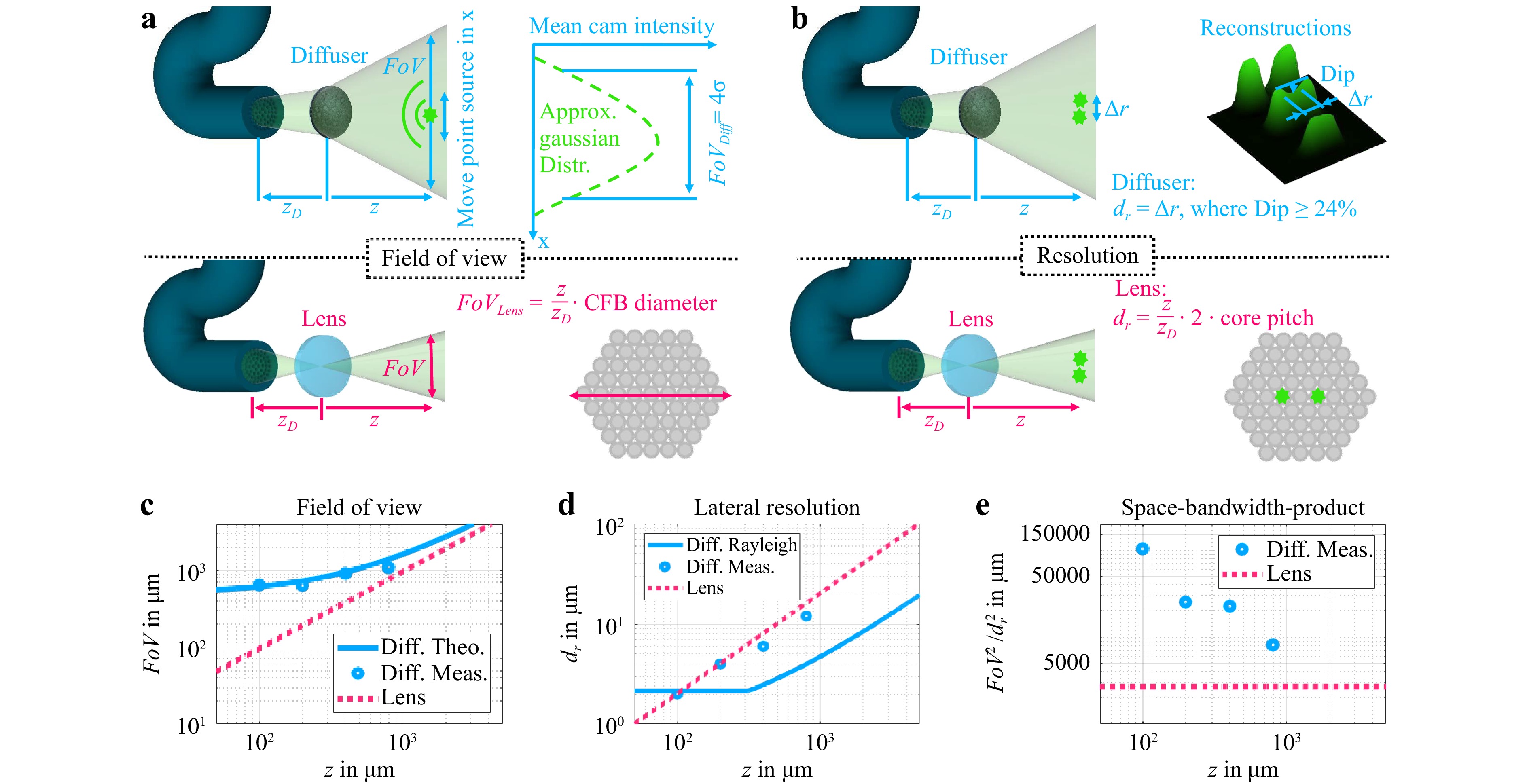
Fig. 5 a Determination of FoV for diffuser endoscope (top) and equivalent lens system (bottom). The refractive power of the lens is assumed to vary in such a way that the conjugate plane of the facet is always at the object distance z. b Determination of lateral resolution for diffuser endoscope (top) and equivalent lens system (bottom). The NA of the lens system is assumed to be the core NA. The lateral resolution of the lens system is determined by the magnified core pitch and not the diffraction limit. c Theoretical and measured FoV for the diffuser endoscope and theoretical FoV of equivalent lens system. d Theoretical and measured lateral resolution for the diffuser endoscope and theoretical lateral resolution of equivalent lens system. e Theoretical and measured SBP for the diffuser endoscope and theoretical FoV of equivalent lens system.
A major limitation of the neural network reconstruction is the sparsity of the object scene to reconstruct. Even if training with data of similar sparsity can counteract this effect, the reconstruction quality suffers from non-sparse objects. Less sparse input to the optical system leads to smaller contrast in the speckle patterns that are transferred to the camera by the CFB and thus, to a decreased reconstruction quality. To enhance the speckle contrast, structured illumination could be implemented, e.g. by focusing the illumination laser onto one fiber core on the proximal side, so that the object on the distal side is illuminated by a speckle pattern. By sequentially focusing through different fiber cores, even the information throughput of the system could be further enhanced at the cost of temporal resolution.
For an application in brain diagnostics, the scattering by the tissue is another limitation. Considering a transport mean free path of 900 µm in brain tissue51, our endoscope should be capable of imaging up to such a depth. However, because of the increasing noise due to scattering by the tissue for higher penetration depth, a degradation of reconstruction quality is expected. At the moment, the network reconstruction is only able to correct the scattering by a known diffuser and is susceptible to changes. If the reconstruction scheme could be expanded to random diffusers52, tissue scattering could potentially be decreased too for higher imaging depth.
In the optical setup, the CFB acts as an information bottleneck. For a lens-based endoscope, the space-bandwidth product is limited by the number of fiber cores. For a diffuser endoscope, that limit can be overcome with compressed sensing. The diffuser acts as an encoder to a domain where the information is sparse. Thus, optimizing it to match the problem at hand can potentially improve the imaging capabilities. Currently, a non-optimized random diffuser was mounted on the CFB with a thin glass spacer. This leads to a loss of contrast in the captured images and subsequently to a worse reconstruction by the neural network. Moreover, it has a very small optical memory effect, prohibiting the application of reconstruction approaches that rely on shift invariance. The distal ferrule containing the diffuser and fiber has a diameter of 700 µm, determining the diameter of the endoscope. In principle, the endoscope head could easily be miniaturized to the CFB diameter of 350 µm, but it would also limit the achievable FoV. In the future, optimization of the diffractive optical element on the distal side of the fiber bundle could enhance the imaging capabilites further. Furthermore, the diffuser could be realized as a 3D printed microlens array on top of a gradient-index (GRIN) lens39 or even a random phase mask as part of a deep optical system where the optical encoder and the neural network decoder are part of an end-to-end optimization54, 55. The neural network architecture could be refined by using a physics-informed network layer modeled after the point spread functions in the FoV for spatially varying deconvolution56. This would also allow reconstruction with higher resolution, as less learnable parameters would be required. Deep learning techniques for super-resolution in fluorescence microscopy could be applied as well57. Furthermore, a perceptual loss function based on a second network pretrained for image classification could be employed. In comparison to conventional loss functions, it could measure the differences between the reconstructed and the ground truth images in a way that is closer to human perception58, 59. After optimization of the optical setup and image reconstruction with the discussed steps, the improved imaging quality could enable previously impossible in vivo applications outside of lab experiments.
-
To describe the optical system, a simple forward model60
$$ {\bf{y}}={\bf{H}}{\bf{x}} $$ (1) can be applied, where $ {\bf{y}} $ is the $ M\times1 $ flattened measured image vector and $ {\bf{x}} $ is the $ N\times1 $ flattened object space vector. $ {\bf{H}} $ is the $ M\times N $ transmission matrix, which can be derived from calibration measurements. For megapixel diffuser camera setups, $ {\bf{H}} $ can become very large, so high computational power, memory and calibration effort are necessary. Separable61, 62 or convolution-based63, 64 forward models can be applied to reduce the calibration effort and computational complexity by several orders of magnitude60. However, separable forward models do not work with arbitrary diffusers, and special phase mask designs with low fabrication tolerances are needed. Convolution-based forward models rely on the shift invariance of the PSF of the diffuser65, which significantly reduces the effective FoV. By measuring multiple PSF in one object plane, the effective FoV can be enlarged, thus creating a shift variant forward model66.
Miniaturized CFB only have several thousand fiber cores, so that $ M $ can be chosen small enough to directly apply the forward model from Eq. 1. Since usually $ M<N $, the equation system in Eq. 1 is underdetermined and therefore has an infinite amount of solutions. A common method for object reconstruction is to solve a convex optimization problem60
$$ {\bf{\hat{x}}}=\text{argmin}_{\bf{x}} \|{\bf{y}}-{\bf{H}}{\bf{x}}\|_2^2+\lambda R({\bf{x}}) $$ (2) where $ \lambda $ is a Lagrange multiplier. The regularizer $ R $ determines the properties of the solution $ \mathbf{\hat{x}} $ and must be chosen according to a priori knowledge about the imaged object x. In case of fluorescence imaging, Eq. 2 can be optimized for sparsity by choosing $ R $ to be the $ L_1 $ norm60. Convex optimization is an iterative and time-consuming approach, which impedes video rate imaging. By employing neural networks for the image reconstruction, the imaging rate can be drastically increased.
For the purpose of parameter studies, the imaging part of the system was simulated by angular spectrum propagation67. The object image is divided into pixels/voxels which are approximated as point sources (Fig. 3). For each point source, a spherical wave is then propagated through the diffuser, which is modeled as a random phase mask. This mask is then applied to the electrical field distribution before angular spectrum propagation is employed to propagate the field onto the distal side of the CFB and to retrieve the corresponding PSF of the pixel/voxel. The intensity pattern on the distal fiber facet for a certain object is then retrieved by superposition of the PSFs of all illuminated pixels/voxels of the object weighted by their intensity. To simulate the transmission of the intensity pattern through the fiber, a fiber bundle simulator developed at the University of Kent53 was used to imitate the Fujikura fiber we used in our lab experiments.
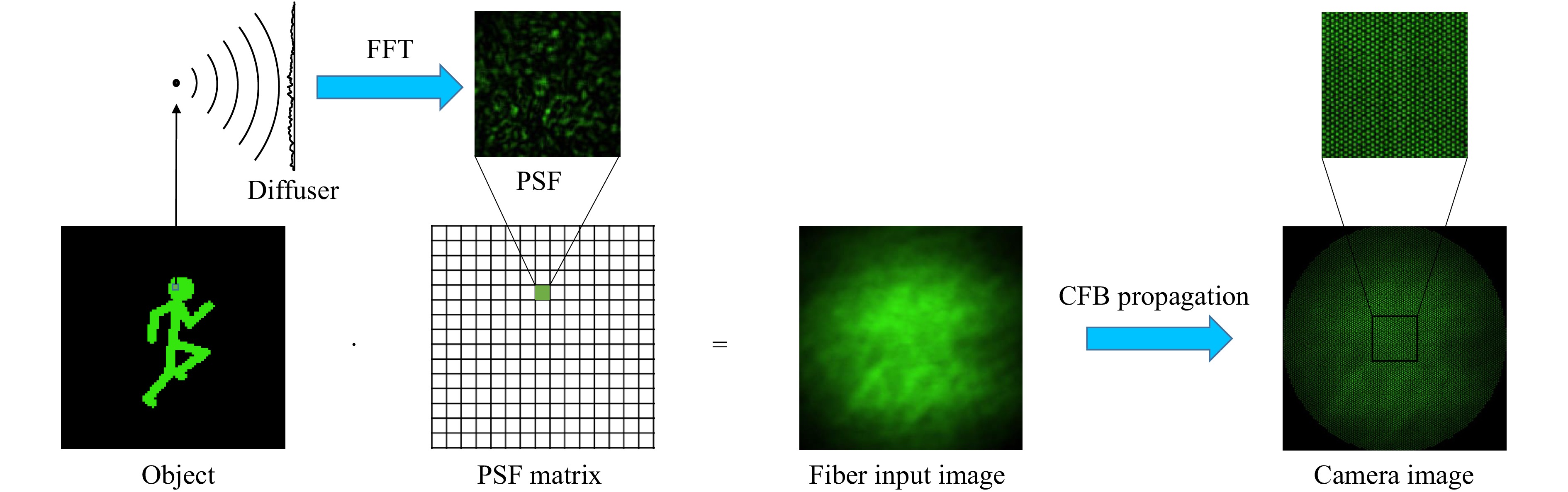
Fig. 3 Simulation of optical system. The object image is encoded with diffuser by superposition of PSFs for illuminated pixels/voxels: For each pixel/voxel in the FoV a PSF is calculated using Fourier Optics. The speckle pattern is then calculated by superposing each PSF weighted by the intensity of the corresponding object pixel/voxel. The transmission through the CFB is simulated with a fiber bundle simulator53.
-
In the optical setup for fluorescence imaging, as shown in Fig. 1a, the illumination laser with a wavelength of 488 nm is reflected into the CFB with a dichroic beamsplitter. The illumination light is guided through the CFB and the diffuser to the imaging volume, which contains fluorescent particles emitting incoherent light. The fluorescence light is then scattered by the diffuser. It consists of diffuse tape mounted onto a cylindrical glass spacer with a length of 500 µm which is glued to the distal end of the CFB. The glass spacer and the CFB are enclosed by a metal ferrule determining the total endoscope diameter of 700 µm. The specifications of the diffuser endoscope head are displayed in the following section. The used diffuser acts as a random phase mask and encodes the object image into a speckle pattern. This pattern is then propagated onto the distal facet of the coherent fiber bundle, a Fujikura FIGH-10-350S with 10000 fiber cores on a 325 µm image diameter. The intensity information of the speckle patterns is transmitted onto a Thorlabs Quantalux CS2100M camera on the proximal side of the fiber through the fiber cores, which have a diameter of 1.7 µm and a mean core pitch of 3.1 µm. The shift invariance of the diffuser endoscope was investigated by laterally shifting a point source over the FoV and examining the correlation coefficient between the captured PSF and the PSF at the zero position. The lateral optical memory effect was calculated by using the full width at half maximum (FWHM) of a gaussian curve fit onto the correlation coefficients of the shifted PSFs. For z = 200 µm, it was determined at approximately 50 µm, which roughly equals a tenth of the measured FoV.
To gather a large number of training images with the experimental optical setup, a Texas Instruments DLP4710 digital light projector (DLP) including an RGB LED is employed to project different ground truth data with a resolution up to 1920 × 1080 into the object space (Fig. 4). To achieve the correct demagnification of the object images, the projection optics of the DLP were replaced by an 180 mm Olympus tube lens and an Olympus plan achromat microscope objective with a 40 × magnification and an NA of 0.61. For the acquisition of 3D training data, the DLP is moved along the depth axis with a linear stage to introduce images from different distances to the diffuser endoscope.
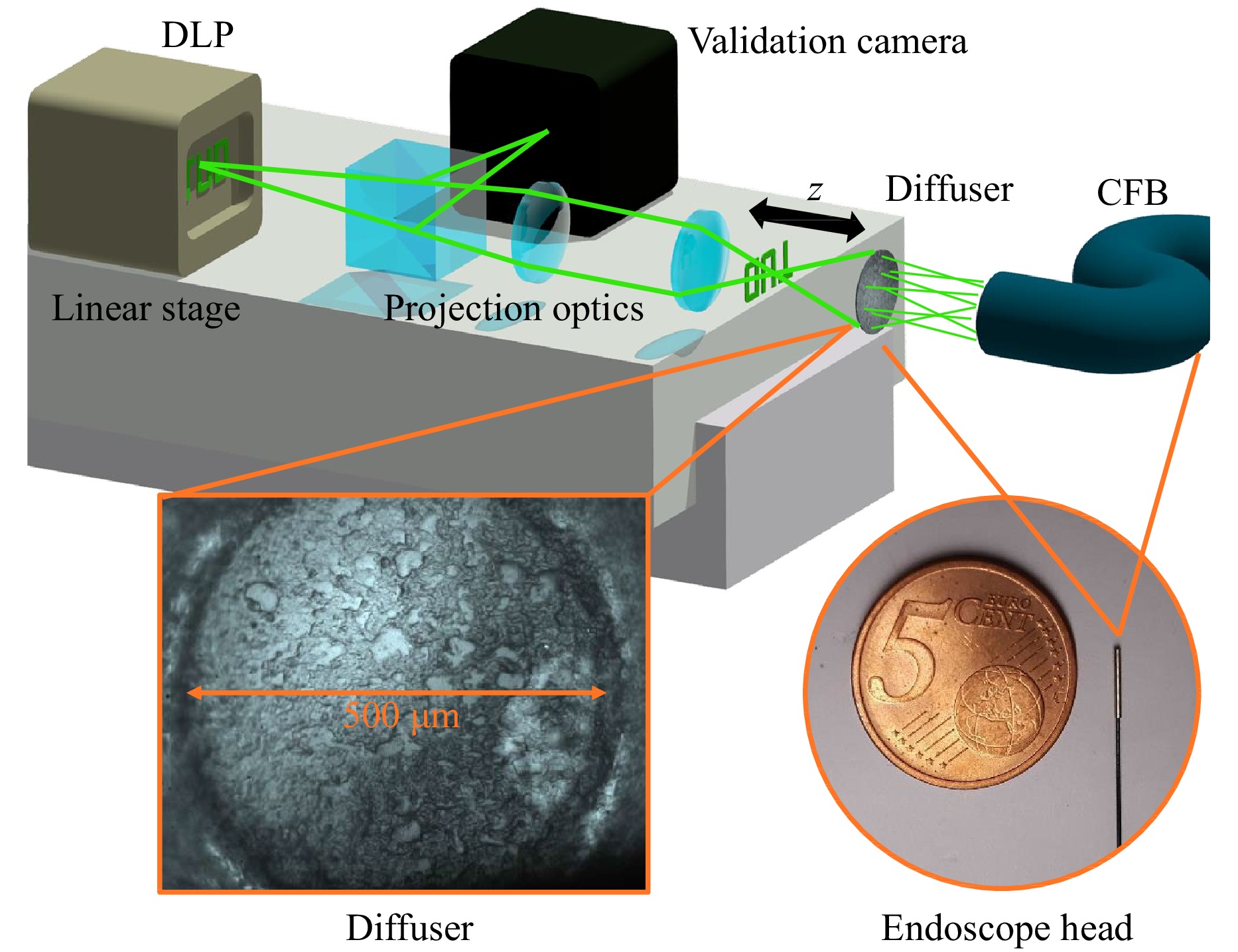
Fig. 4 (top) Training Setup. A digital light projector (DLP) on a stage is employed to project training images from different depths into the optical system and onto a validation camera. (bottom left) Diffuser surface captured by the validation camera. (bottom right) Comparison of the thin probe tip with a diameter of 700 µm to a coin.
The fluorescence images in Fig. 2b show agglomerations of Rhodamine B marked Melamin resin particles with a diameter of 10 µm, placed on a cover glass. For the 3D imaging shown in Fig. 2e, particles were placed on the front and back surface of the cover glass. The thickness and refractive index of the cover glass were 0.17 mm and 1.53, respectively (ISO 8255-1:1986), resulting in an optical path distance of 0.26 mm between the front and back surface.
-
The diffuser endoscope’s FoV and lateral resolution are compared to an endoscope where the diffuser is replaced with a paraxial lens at the same distance to the CFB. The theoretical lateral FoV of the diffuser endoscope is defined as
$$ FoV({\textit z})=\min[w,l+2\cdot {\textit z}_{\rm{D}}\cdot \tan\alpha_{\rm{C}}]+2\cdot {\textit z}\cdot \tan\alpha $$ (3) where
$$ \alpha_{\rm{C}}=\sin^{-1}\frac{A_{\rm{NC}}}{n} $$ (4) is the light acceptance angle of the fiber cores, $ l $ the CFB diameter and $ w $ the diffuser diameter (Fig. 6).
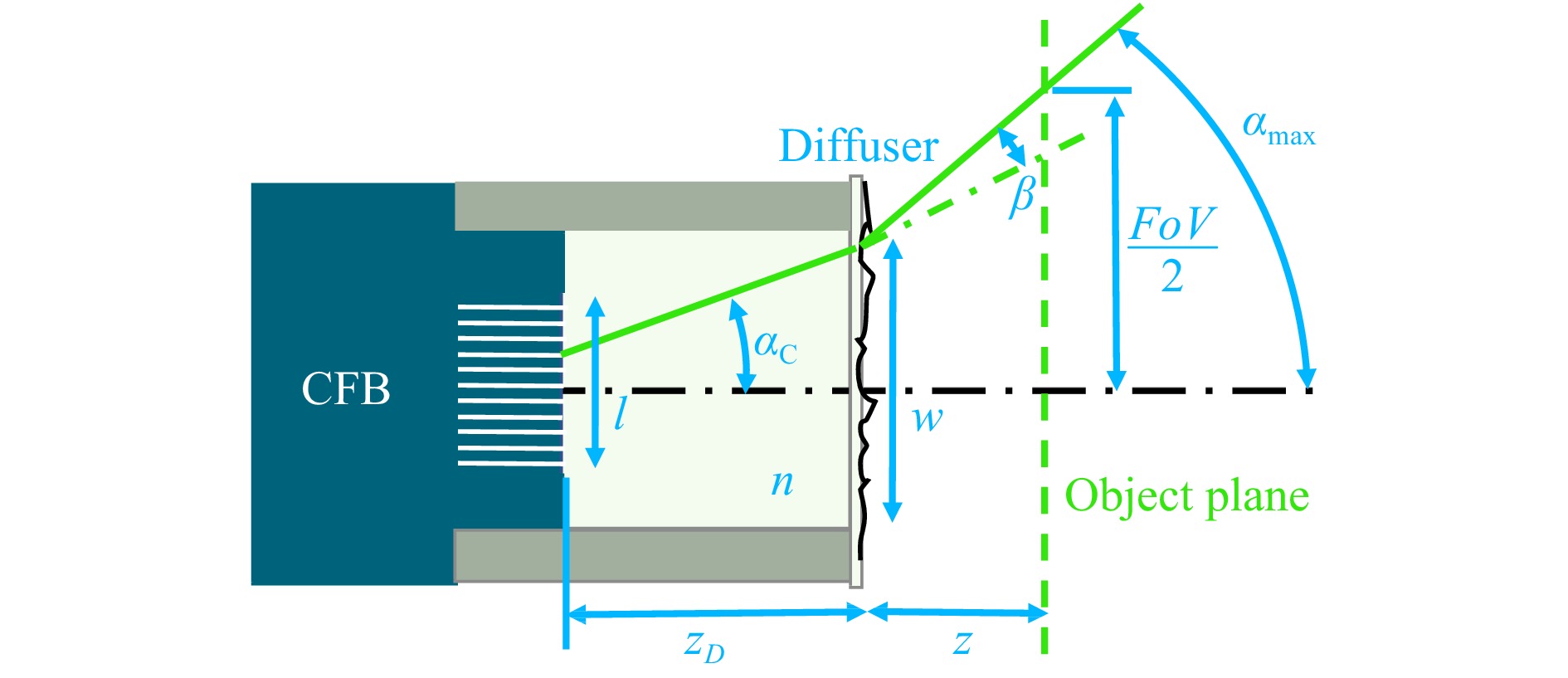
Fig. 6 Diffuser endoscope head. The $ FoV $ is determined by the object distance z and the maximum angle $ \alpha_{\rm{max}} $ from which light can enter the cores of the CFB. $ \alpha_{\rm{max}} $ is increased by the diffuser stray angle $\, \beta $ and is either limited by the light acceptance angle of the fiber cores $ \alpha_{\rm{C}} $ or by the properties of the endoscope head, including the CFB diameter $ l $, the glass spacer length $ z_{\rm{D}} $ and refractive index $ n $ as well as the diffuser diameter $ w $.
The maximum angle of light acceptance $ \alpha $ is defined as
$$ \alpha=\beta+\sin^{-1}(n\cdot\sin\alpha_{\rm{min}}) $$ (5) with
$$ \alpha_{\rm{min}}=\min\left[\alpha_{\rm{C}},\tan^{-1}\left(\frac{l+w}{2\cdot {\textit z}_{\rm{D}}}\right)\right] $$ (6) The stray angle β was defined as twice the standard deviation of a gaussian curve fitted to the stray angle spectrum. The stray angle spectrum was measured by illuminating the diffuser tape with a collimated beam and capturing the far field onto a camera. The FoV of the diffuser endoscope was additionally determined experimentally as the lateral object distance from which light is captured into the CFB (Fig. 5a, top).
The theoretical and experimental results of the diffuser endoscope’s FoV are in good agreement. An offset of the diffuser diameter magnitude at zero axial distance is visible (Fig. 5c). In contrast, the FoV of the lens endoscope is proportional to the axial distance and goes down to zero at z = 0. Hence, the diffuser endoscope has an inherently larger FoV in the near field.
A theoretical limit for the lateral and axial resolution is given by the object sided numerical aperture of the system in air
$$ A_N=\sin u_{max} $$ (7) It is defined by the maximum angle $ u_{max} $, from which light from an object on the optical axis can enter the CFB
$$ u_{max}=\min\left[\tan^{-1}\left(\frac{\min[w_D,w]}{2\,{\textit z}}\right),\alpha_C+\beta\right] $$ (8) Here $ w_d $ is the ray intersection diameter at the diffuser for the case of an infinitely large core NA is defined as
$$ w_D=l-\frac{2\,{\textit z}_D}{n}\cdot\tan\left(\tan^{-1}\left[\frac{l/2}{{\textit z}+{\textit z}_D/n}\right]-\beta\right) $$ (9) For the values given in Table 2, the NA is limited by the fiber core aperture angle $ \alpha_C $ at z < 300 µm and by the stray angle β at larger distances. For the fluorescence wavelength λ = 0.65 µm, a lateral resolution 1.2$ \cdot\lambda/A_N $ of (2...4) µm and an axial resolution $2 \cdot\lambda/A_N^2 $ of (10...32) µm can be achieved within the measurement volume according to the Rayleigh criterion.
Quantity Symbol Magnitude Metal ferrule diameter 700 μm CFB diameter l 350 μm Core NA68, 69 ANC 0.39 Core diameter69 1.7 μm Core open area ratio69 0.21 Core pitch69 3.4 μm Refractive index of glass spacer n 1.5 Diffuser-CFB distance zD 500 μm Diffuser diameter w 500 μm Diffuser stray angle (2σ) β 6.2° Table 2. Specifications of the diffuser endoscope head.
Analogously, the diffuser endoscope’s lateral resolution was experimentally determined by the distance between two points at which the intensity between the points drops by 24% (Fig. 5b). In case of the lens endoscope, two points are distinguishable in the CFB plane if there is at least one non-illuminated core between them. The lateral resolution of the diffuser endoscope and the lens endoscope have similar magnitudes and are both proportional to the axial distance of the system (Fig. 5d). This implies that the lateral resolution of the diffuser endoscope is also limited by the core pitch and the magnification $ {\textit z}/{\textit z}_D $. The diffuser endoscope is diffraction limited at z = 100 µm (Fig. 5d). At larger distances, the magnified core pitch limits the two point resolution. The space-bandwidth-product (SBP) is defined as the squared quotient of the FoV and the lateral resolution. While the SBP of the lens endoscope is bound to the core number and therefore constant, the SBP of the diffuser endoscope increases with decreasing object distance, leading to an inherent imaging advantage in the near field (Fig. 5e). At an axial distance of 100 µm it exceeds the constant lens endoscope SBP by a factor of 38.
To determine the axial resolution experimentally, the intensity share curves in Fig. 2c were differentiated. The axial resolution was then defined as 2$ \sigma $ of the resulting peaks in approximation to the Rayleigh criterion. Within the measurement volume, the axial resolution ranges from 13 µm to 32 µm, depending on the object distance, which is in good agreement with the theory above.
Further improvement of the spatial resolution are possible, e.g. by increasing the stray angle of the diffuser. Furthermore, the fiber-facet-diffuser distance $ {\textit z}_D $ can be adapted to match the magnified core pitch to the diffraction limit at other distances.
-
For the image reconstruction, two neural networks are trained sequentially. The first network is a Single Layer Perceptron (SLP), which consists of a single fully connected layer with weights and biases between all pixels of the input and the output layer. Moreover, the activation function was omitted, so that the network represents the pseudo-inversion of the intensity transmission matrix H from the linear forward model in (1). However, some artifacts remain in the background due to non-linearities in the optical system. Thus, the trained SLP is used to generate training data for a second network, a slightly modified U-Net, which serves as denoising network to clean up the artifacts arising from the intermediate SLP reconstruction. While the U-Net was originally developed for image segmentation70, it can easily be adapted to be applicable for image-to-image regression by replacing the output layer. The employed U-Net was comprised of three encoding and decoding stages for the 2D and 3D reconstruction. For both networks, the loss function used for training is the mean squared error (MSE) between the reconstructed image and the ground truth. The reconstruction scheme is displayed in Fig. 7a. For all network trainings, an Adam optimizer71 with a learning rate of 10−4 and a mini-batch size of 32 were used. As a convergence criteria, validation patience was employed, where the training is stopped after a certain number of validation iterations have passed without an improvement in the validation loss. For this paper, validations were calculated every 20 iterations and the training was stopped after 200 validations without improvement for the SLP and 100 validations for the U-Nets.
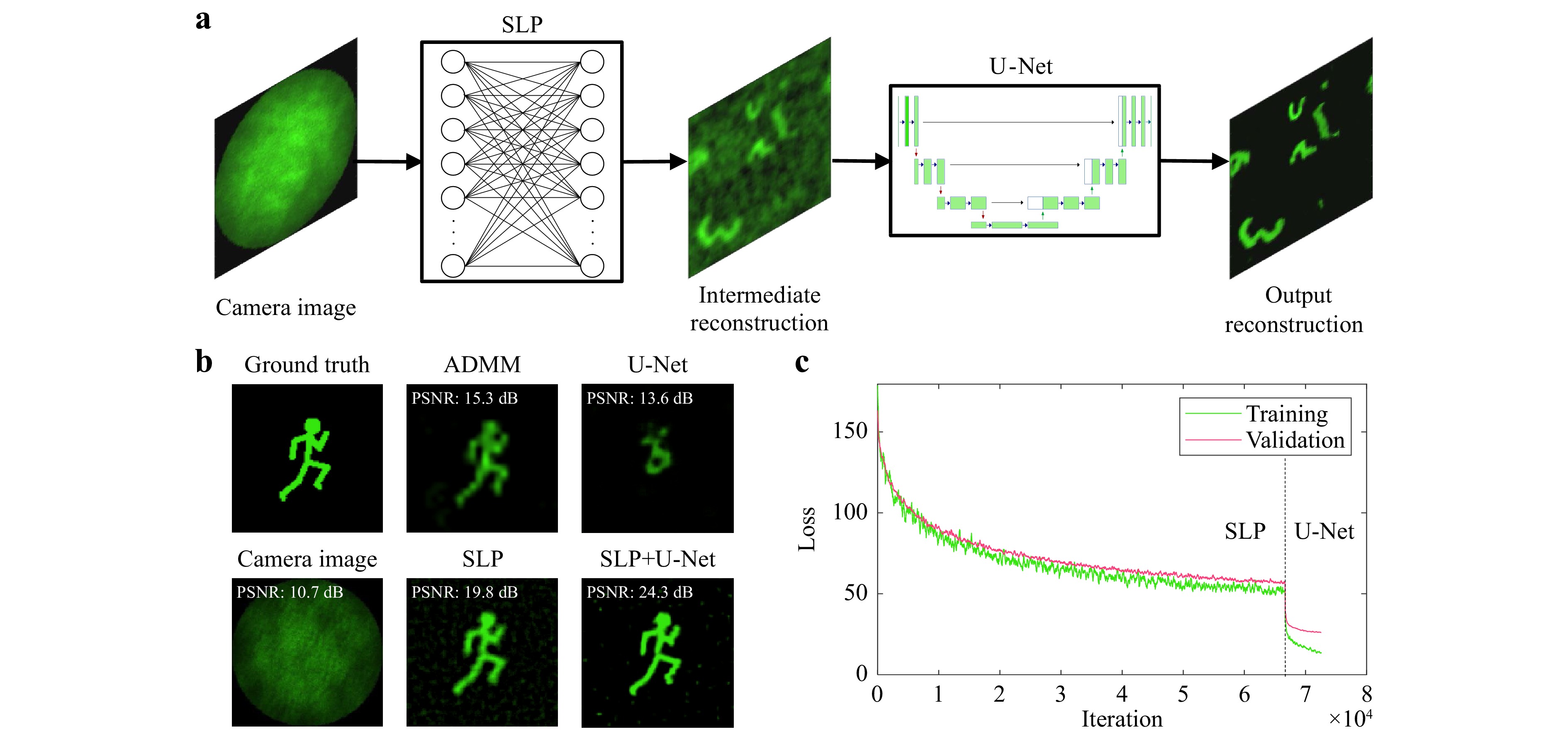
Fig. 7 a Neural Network Architecture for image reconstruction. The input measurement is fed into a Single Layer Perceptron (SLP) which is trained with Augmented MNIST digits so that the learned weights represent the inverse of the optical transfer function. The intermediate reconstruction is then denoised by a U-Net to retrieve the final output. The networks are trained separately. The training input of the U-Net are the predictions of the training data by the SLP. b 2D Reconstruction of “Running Man” test data with different approaches. Top, from left to right: Ground Truth Image. Reconstruction by iterative ADMM algorithm40. Reconstruction by single U-Net. Bottom, from left to right: Simulated Camera Image. Reconstruction by Single Layer Perceptron (SLP). Reconstruction by combination of SLP and U-Net. c Training and validation loss progress for SLP and U-Net.
The performance of the combination of SLP and U-Net as well as each network alone is compared to the iterative ADMM algorithm introduced for a diffuser-based camera40 in Fig. 7b for “Running Man” test data which differs from the “Augmented Digits” training data. The reconstruction quality is also examined with different metrics in Table 3 as a cross-validation for “Augmented Digits” training and test data. While the ADMM algorithm is capable of reconstructing images scattered by a diffuser with high fidelity given a sufficiently large memory effect, the addition of the CFB disturbs its reconstruction capabilities significantly. Due to the implemented regularization, the reconstruction is sparse, especially in the outer image are where the memory effect is not high enough. This leads to a rather high SSIM even if the correlation coefficient indicates a very bad result. The U-Net alone suffers from bad generalization and fails to extract features from the speckle patterns. The dark parts of the image are reconstructed accurately, resulting again in a misleadingly high SSIM. The SLP, on the other hand, is generalizing very well and is capable of reconstructing most of the features from the ground truth image, however, the output image is blurry and contains some background noise leading to a low SSIM. With the help of the U-Net applied to the SLP output, this effect can be reduced significantly to retrieve a reconstruction with high fidelity. Furthermore, the reconstruction by the two consecutively applied neural networks is about 200 times faster than the iterative ADMM reconstruction approach. The combination of SLP and U-Net also outperforms the single networks as well as the ADMM algorithm in all metrics.
Metric ADMM U-Net SLP SLP+U-Net Test Train Test Train Test Train Test PSNR 17.3 ± 2.5 dB 23.0 ± 4.3 dB 22.2 ± 4.7 dB 23.1 ± 2.8 dB 22.5 ± 3.1 dB 28.8 ± 3.3 dB 26.4 ± 4.3 dB SSIM 0.73 ± 0.07 0.67 ± 0.15 0.65 ± 0.16 0.30 ± 0.06 0.28 ± 0.06 0.92 ± 0.04 0.89 ± 0.06 CC 0.09 ± 0.14 0.79 ± 0.08 0.75 ± 0.09 0.78 ± 0.10 0.76 ± 0.11 0.94 ± 0.04 0.90 ± 0.05 Time 1541 ± 28 ms 4.5 ± 2.5 ms 2.9 ± 2.5 ms 7.4 ± 4.8 ms Table 3. Comparison of reconstruction approaches for “Augmented Digits” data with cross-validation results for neural networks. Values are given with $ 1\sigma $ standard deviation.
The dataset “Augmented Digits” is comprised of 10000 pairs of ground truth and speckle images for training as well as 1000 image pairs for validation and testing. The ground truth images are created by randomly selecting up to five images from the MNIST Digit dataset (28 × 28 pixels), randomly shifting, scaling and rotating them, and placing them randomly in the final image of 104 × 104 pixels. A reconstructed example can be seen in Fig. 7a (right). For 3D ground truth images, the samples from the MNIST digits dataset are placed at a random depth chosen from a set of layers (Fig. 2d). All network training and testing was performed on an NVIDIA RTX A6000 GPU of our workstation.
-
This work was supported by the German Research Foundation (DFG) under grant (CZ 55/48-1).
Single-shot 3D incoherent imaging with diffuser endoscopy
- Light: Advanced Manufacturing 5, Article number: (2024)
- Received: 13 September 2023
- Revised: 01 March 2024
- Accepted: 05 March 2024 Published online: 30 May 2024
doi: https://doi.org/10.37188/lam.2024.015
Abstract: Minimally invasive endoscopy offers a high potential for biomedical imaging applications. However, conventional fiberoptic endoscopes require lens systems which are not suitable for real-time 3D imaging. Instead, a diffuser is utilized for passively encoding incoherent 3D objects into 2D speckle patterns. Neural networks are employed for fast computational image reconstruction beyond the optical memory effect. In this paper, we demonstrate single-shot 3D incoherent fiber imaging with keyhole access at video rate. Applying the diffuser fiber endoscope for fluorescence imaging is promising for in vivo deep brain diagnostics with cellular resolution.
Rights and permissions
Open Access This article is licensed under a Creative Commons Attribution 4.0 International License, which permits use, sharing, adaptation, distribution and reproduction in any medium or format, as long as you give appropriate credit to the original author(s) and the source, provide a link to the Creative Commons license, and indicate if changes were made. The images or other third party material in this article are included in the article′s Creative Commons license, unless indicated otherwise in a credit line to the material. If material is not included in the article′s Creative Commons license and your intended use is not permitted by statutory regulation or exceeds the permitted use, you will need to obtain permission directly from the copyright holder. To view a copy of this license, visit http://creativecommons.org/licenses/by/4.0/.

 DownLoad: