FPGA-accelerated mode decomposition for multimode fiber-based communication

The advent of multimode fibers (MMFs) has significantly enhanced the capacity and efficiency of optical communication systems, addressing the escalating demand for higher data rates and bandwidth^1,2. MMFs exploit multiple spatial modes within a single fiber core, allowing the simultaneous transmission of multiple data streams, thereby increasing the fiber’s overall capacity³. However, the light transmission within MMFs is complicated by mode coupling, which can affect the fiber’s performance by inducing unwanted interactions among modes^4,5, see Fig. 1. In classical communication, mode crosstalk is corrected at the receiver side through complex digital signal processing⁶. Instead, channel distortion should be compensated in advance for quantum key distribution (QKD). Accurately obtaining the spatial modes of MMFs is therefore essential for both fundamental research and practical applications. The characterization of the transmission properties of MMF offers the chance to integrate a closed-loop control (CLC) system for applying digital pre-coding in communication and in fiber imaging systems⁷⁻⁹.

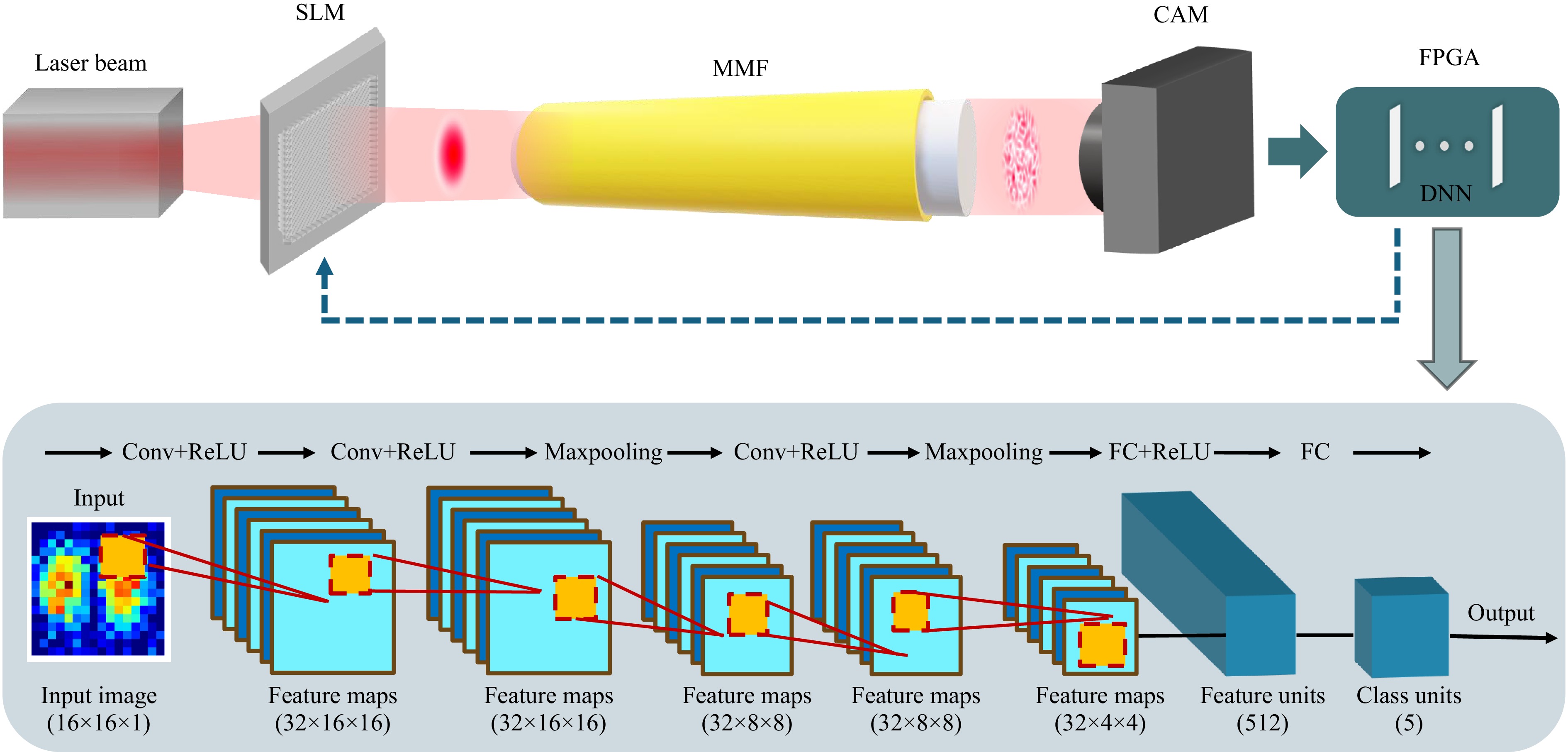
Fig. 1  Schematic of optical fiber crosstalk and the pipeline of FPGA-based mode decomposition for a CLC system. Abbreviations: CAM: camera; SLM: spatial light modulator. An input Gaussian beam is converted into multiple modes during propagation through the MMF, resulting in a complex speckle pattern for coherent light. The speckle pattern is then sent to an FPGA running a deep neural network for analyzing the modal content. An 11-layer CNN model for mode classification. Here, 5-mode is taken as an example. Input is a gray value image with a resolution of . The output is the probability corresponding to each pattern category. The specific operations of each layer are shown above the box.

Mode decomposition (MD) refers to a technology that quantitatively decomposes the output of an MMF, known as speckle patterns, into individual transverse eigenmodes including amplitude and phase weights for each polarization. In general, MD can be divided into two different categories: optical methods and numerically computational methods. Optical methods of MD in MMFs as a solution to the well-posed inverse problem, such as digital holography (DH) algorithms^10,11, and optical correlation filters^12,13, often involve complex hardware configurations. While effective, these methods tend to be limited by their scalability, unstable phase drifts over long fibers, and real-time processing capabilities¹⁴. Consequently, there is a growing interest in leveraging advanced computational techniques, such as deep neural networks (DNNs)^4,15−17, Gerchberg-Saxton (GS) algorithm¹⁸, Stochastic Parallel Gradient Descent (SPGD) algorithm¹⁹, to enhance the efficiency and accuracy of MD in MMFs.

Among these, DNN-based MD is becoming one of the main streams of the solution of the ill-posed problem and is preferred in the case of fewer modes due to their relative simplicity. By learning the mapping between beam patterns and mode coefficients (amplitude and phase) from a vast dataset, deep learning techniques can perform the MD process. Employing a trained CNN can accomplish MD tasks in milliseconds, significantly enhancing time efficiency compared to traditional numerical methods like SPGD. In addition, this method does not require reference light like DH and only uses simple intensity images²⁰. Therefore, this method is welcome in long-haul fiber systems.

Although deep learning has its advantages, running large networks on CPU platforms is often impractical due to insufficient computational resources. GPUs, preferred for their high computational power and ease of use in development frameworks, face issues related to high energy consumption and low energy efficiency. In this work, FPGAs are emerging as a viable research topic for neural network acceleration. Given the current demand for optimized, energy-efficient CNN models, FPGAs offer a promising avenue for optimizing neural networks and running neural networks on low-power embedded processors while maintaining reasonable network accuracy and reducing computational costs and power consumption²¹. In optical experiments, FPGA also shows the benefit of lower latency compared with personal computers^22,8, such as the applications in correcting distortion for optical imaging²³ and ultrasound flow imaging²⁴.

In this paper, we explore the feasibility, limitations, and advantages of using FPGA to run neural networks for MD. To accelerate the characterization of mode weights, we optimized the generation of the training dataset, eliminating the need for additional steps to recover the phase as required in previous works²⁰. Through simulations and experiments, we verified that FPGA-based quantized neural networks can achieve accurate MD with low power consumption and high efficiency. The proposed approach has the potential to accelerate the deployment of AI-based MDs for MMF, paving the way for more efficient and scalable optical communication systems based on CLC by FPGA. Our results also provide valuable insights for integrating AI-based methods into industrial environments.

In the weakly guiding approximation, the eigenmodes in optical fibers can be represented by the fields in terms of linearly polarized modes, called LP modes²⁵. The transverse optical field in MMF can be considered a linear superposition of all individual LP modes, which can be defined as

where the $ {{\Psi }}_{n\left(x,y\right)} $ is the electric field of the $ {n}_{th} $ eigenmode in the fiber with complex mode weights $ {c}_{n} $ including amplitude weight $ {\rho }_{n} $ nd relative phase $ {\phi }_{n} $. Imperfections in manufacturing, bending, and twisting of the optical fiber primarily cause mode coupling in MMFs. This coupling leads to modes superposition, manifesting as a speckle pattern at the output of the fiber, referred to as a speckle pattern²⁶. MD refers to an approach that allows the complex field distribution to be decomposed into multiple modes with specific complex mode weights. In this work, the intensity distribution of the light field emerging from MMF is used to estimate the mode weights, which can be expressed as follows:

The purpose of this work is to train a neural network that can learn the nonlinear relationship $ S(\cdot) $ between the intensity image and mode weights.

For the presented problem, proper training datasets should be generated to train a neural network successfully. When there is no crosstalk between modes, meaning each output light field distribution corresponds to an eigenmode, MD could be simplified as a classification task that is suitable for low-crosstalk fibers. The LP eigenmode distribution is first generated in a simulation for the mode classification. Considering the background and environmental noise in the real world, random Gaussian noise is added to the synthetic data to create a comprehensive dataset, which is a type of statistical noise with a probability density function equal to that of the normal distribution²⁷. The probability density function φ of a Gaussian random variable z is given by:

where σ represents the mean value, and σ represents its standard deviation²⁸. In this work, the resolution of classification data is set as 16 × 16 from 3 to 40 modes. Each eigenmode contains 100 variants with random Gaussian noise. Therefore, the total amount of images in the dataset is 100 × N.

A more commonly occurring scenario is that the input light is distorted due to intermodal crosstalk and the output light field is a superposition of multiple modes. In this case, one pair of training data including the intensity distribution and complex mode weights is needed for training a neural network to perform MD. Due to the complexity of the combination of modes, a large amount of data is required to accurately train the network for MD. Therefore, a pseudo-random weight combination is used to generate the light field in this work, including generating random amplitude and random phase weights. As the physical energy conservation must be satisfied, the random values of amplitude weights are normalized such that the sum of their squares equals 1.

How to handle phase weights is critical in influencing the successful training of a neural network to perform correct MD. Due to phase ambiguity¹⁸, the phase weights cannot be directly used as labels. The first ambiguity arises because of the same relative phase difference among modes resulting in the same intensity image when the amplitude weights are the same. This occurs when the absolute phase distributions differ, while the relative phase differences between modes remain the same. To solve this issue, the phase of the fundamental mode is set to zero, and only the relative phase differences between higher-order modes and the fundamental mode are considered. This ensures that the phase labels for each intensity image are unique, resulting in a label vector with N-1 phase labels corresponding to N modes.

Moreover, the second ambiguity stems from the conjugate problem, where the same intensity image can have two pairs of phase label vectors with opposite signs. This issue will hinder network convergence. In the previous data-driven neural network to date, the conventional way is to employ the absolute or cos value of the phase as a label^{4,15,16,20,29}. However, the lost phase sign can only be retrieved by brute force search or additional measurements, which are impractical in real applications. To address this, one mode’s relative phase difference is fixed within the range of $ \left[0,{\text π} \right] $ or $ [-{\text π} ,0] $, ensuring unique intensity image labels and enabling the network to learn and predict accurately. In the design, the relative phase difference of the second mode is fixed within the range of $ [0,{\text π} ] $. After generating the amplitude and phase weights, they are combined to produce the intensity images and their corresponding labels. These intensity images are used as the inputs for DNN, and the labels guide the training process.

The presented investigation aims to train a neural network that can be run on an FPGA system to accelerate the decomposition process. In this work, convolutional neural networks (CNNs) were used to classify the eigenmodes and decompose the distal speckle images. Convolutional layers, the core component of a CNN, are often used to process image data to extract valid information from the image with a convolutional operation and pass it to the next layer³⁰. Each convolution operation involves numerous multiplications and additions, which can be efficiently accelerated using the parallel processing capabilities of an FPGA.

In this work, the CNN model is initially trained using PyTorch on a GPU. To deploy this model on an FPGA, it must be adapted due to the architectural differences. This is accomplished using Xilinx Vivado High-Level Synthesis (HLS), which translates high-level C++ descriptions into hardware description languages (HDL). Our approach includes specific annotations to ensure that the generated register transfer level (RTL) precisely aligns with the intended CNN evaluation strategy, controlling all computations and data transfers on a cycle-by-cycle basis. The HLS tool automatically manages the pipelining of the arithmetic units and DRAM transfers. Once the C++ specification is finalized, the HLS tool converts it into RTL, which is then synthesized into an intellectual property (IP) core, ready for integration with the Xilinx FPGA.

This design uses a heterogeneous computing architecture based on Zynq SoC, taking full advantage of hardware acceleration to improve the efficiency of CNN reasoning. Computation-intensive tasks such as convolutional layers and pooling layers are offloaded to the hardware accelerator on the programmable logic (PL) side, while the calculation of the fully connected (FC) layer is performed on the processing system (PS) side. Specifically, convolution and pooling operations are executed using 16-bit fixed-point arithmetic on the PL, whereas the FC layer is processed using 32-bit floating-point arithmetic on the PS. The block design of the acceleration system is shown in Fig. 2a and the pipeline of the implementation of a CNN model to FPGA is given in Fig. 2b.

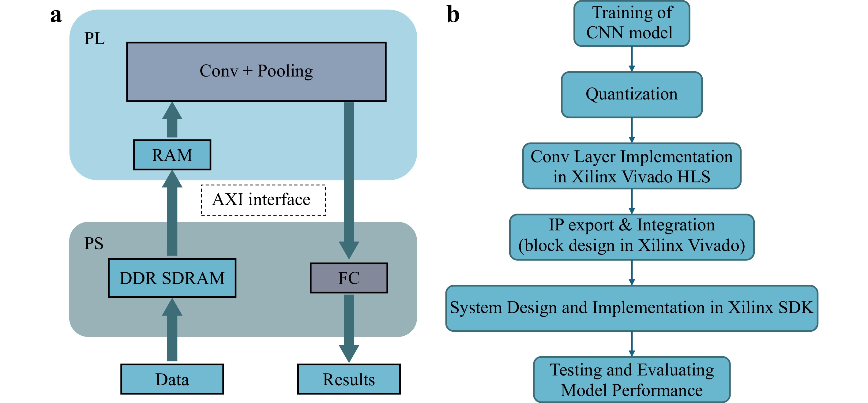
Fig. 2  Overview of the FPGA System design. a The block design of the acceleration system. b The pipeline of the implementation of a CNN model to FPGA.

This design, based on the approach described in³¹, implements efficient hardware acceleration by processing convolutional layers of a CNN sequentially. The architecture employs pipeline execution and double-buffering (ping-pong buffering) techniques to enable concurrent data loading and computation, thus minimizing idle time and enhancing computational throughput. Input feature maps and convolution kernel weights are handled in blocks within the on-chip cache, leveraging loop unrolling and array partitioning to enable parallel computation across multiple convolution kernels. This significantly improves the utilization of hardware resources. Furthermore, zero-padding is incorporated directly during the data loading phase, eliminating the need for additional preprocessing overhead. The convolution computation is optimized through a carefully arranged loop nesting strategy, which maximizes pipeline efficiency while mitigating data dependency challenges. To further enhance performance, the design applies pipeline parallelization during the ReLU activation function, followed by max pooling operations to reduce data dimensionality and minimize external memory access. The key optimization of this design lies in the seamless integration of multi-layer convolution computations using the ping-pong buffering mechanism. This allows for continuous execution of multiple convolution layers along the same data path, reducing intermediate data transfers and significantly improving overall computational efficiency.

After designing the hardware accelerator for the convolutional layers, the custom IP core was integrated into the Zynq SoC platform, with the PS configured to enable efficient communication between the PS and PL through the AXI interface. Once the hardware setup was completed, the system was ready for execution. In the implementation, convolutional and pooling operations are offloaded to the hardware accelerator on the PL side, while the PS is responsible for control, data management, and handling the FC layer. Test data and CNN model parameters are loaded from the SDRM, and floating-point data is quantized into fixed-point format. The hardware accelerator efficiently processes the convolutional and pooling layers, while the FC layer is computed on the PS. Finally, the predictions are yielded. This architecture allows for efficient parallel execution of key CNN tasks, enhancing system performance and ensuring seamless interaction between the PS and PL for data conversion and cache management.

The CNN model was first implemented in Python using the PyTorch package. In this work, the model has been trained and tested from 3 to 40 modes. With a resolution of 16 × 16, the CNN model can achieve nearly 100% accuracy within 30 modes. However, as the number of modes increases, the performance of classification gradually decreases. For the test case of 40 modes, the classification accuracy has dropped to 97.5%. Afterward, the network parameters are quantized and implemented into the FPGA. The results obtained using fixed-point numbers in FPGA and floating-point numbers in PyTorch show the same performance. There is no loss caused by the quantization. This means that the quantization approach used in this work provides a good guarantee of classification accuracy. The test results of using synthetic data on FPGA-based CNN are given in Fig. 3. Taking the 6-mode case as an example, the training process of the model and 2 examples are shown in Fig. 4. As can be seen from Fig. 4a the training loss and validation loss are dropping fast. Both are close to 0 after about 10 epochs. The gap between the training loss and the validation loss is very small, indicating that the CNN model performs consistently on both the training and validation data. This consistency suggests there is no obvious overfitting, even when noise is added. The training curve shows the model has good generalization ability and can maintain high performance on unknown data.

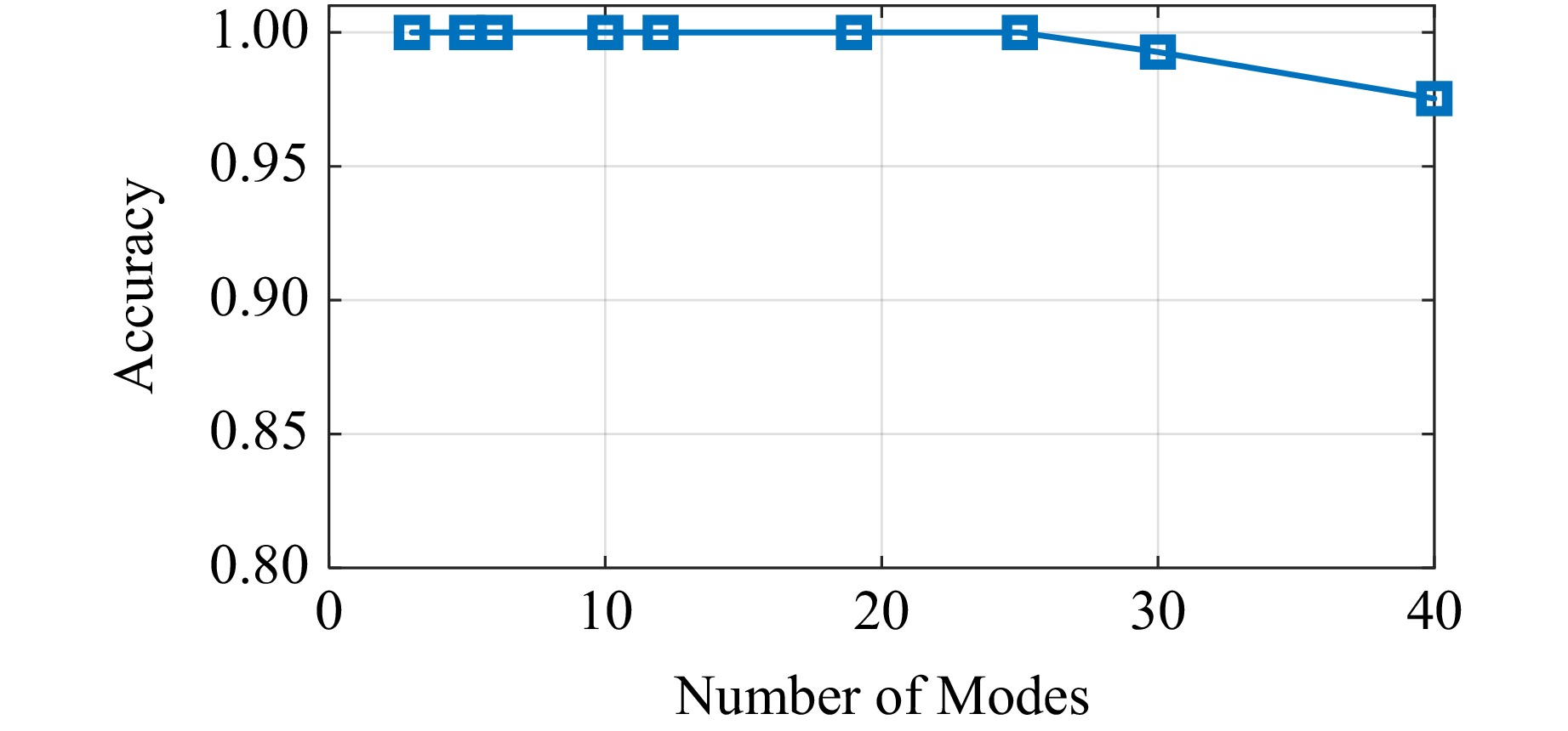
Fig. 3  Performance of FPGA-accelerated CNN on different number of modes classification.

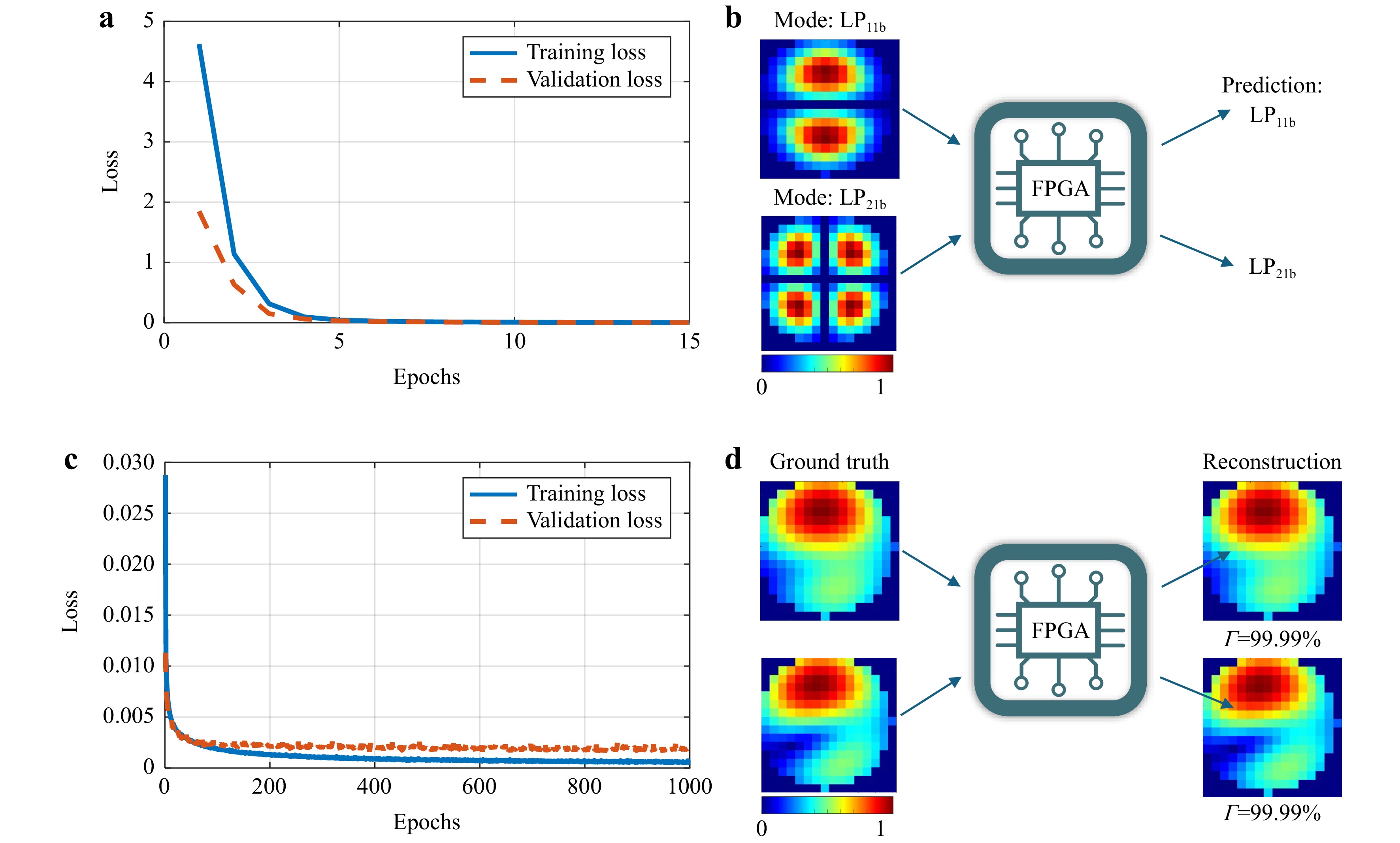
Fig. 4  a Visualization of CNN model training progress for 6-mode classification. b Examples of mode lassification. c Visualization of CNN model training progress for 3-mode decomposition. d Examples of MD (3 modes).

The performance of FPGA-accelerated CNN on MD is investigated in 3 modes. Fig. 4c shows the training loss and validation loss during the training of the CNN model. It can be observed that the loss curve drops sharply in the first few epochs, indicating that the model converges quickly. Its rate of decline slows down over time and eventually approaches zero. Overall, the loss curve is stable in the middle and late stages of training, without obvious fluctuations, which means that the training process is stable and there are no major adjustments or oscillations in the model parameters.

In this work, 1000 samples are used in each test case. The test results from both PyTorch and FPGA for a performance comparison are given in Table 1. It can be found that the network trained in PyTorch provides a precise decomposition on 3 modes, where the average correlation coefficient has a value of 99.52%. The STD of 1000 test samples is 0.0522. The quantized model run in FPGA shows totally the same level of performance with the same mean correlation and standard deviation, which indicates that there is no performance drop. The prediction of amplitude and phase weights shows high accuracy prediction where the amplitude weights error (AWE) is 0.0063 and the phase weights error (PME) is 0.0223. This demonstrates the model’s high accuracy and consistency in reconstructing images from the predicted labels, indicating its strong performance on the test dataset.

Furthermore, decomposition with different numbers of modes is tested on 5 and 6 modes. The corresponding architecture of the CNN model varies with the number of modes. This design ensures that the network has enough capacity to learn more feature details, thereby improving the performance of the MD. In addition, in order to better capture and distinguish the details of different modes, higher resolution images are used, which maintain more detail of the light field distribution. These adjustments improve the network’s ability to recognize different modes, thereby ensuring the accuracy and reliability of the model. As given in Table 1, the results of the decomposition on both 5 and 6 modes show a degradation, where the mean correlation is still around 95% and 90%, respectively.

An optical setup is designed to collect experimental test data, and a simplified representation of the setup is shown in Fig. 5. In this experiment, a laser with integrated single-mode fiber (CoBrite-DX1, Tunable Laser, wavelength =1550 nm) serves as the light source. After collimating the SMF output beam by using a collimator (COL), the beam illuminates the spatial light modulator (SLM) for tailoring the input light field of fiber. A polarizer and a half-wave plate are used to select and adjust the polarization of the beam to meet the requirements of the SLM. The modulated light beam is then guided into a MMF (THORLABS M68L02 – 25 μm, 0.1 NA) through a 4F system including a microscope objective and a lens. The output beam of MMF is imaged onto a camera (CAM1 AVT G1-130 VSWIR) through another 4F system. At the wavelength of the light source used, the fiber supports 3 LP modes per polarization. It should be noticed that a polarizer is placed at the output side of the MMF to filter the same polarization as the input.

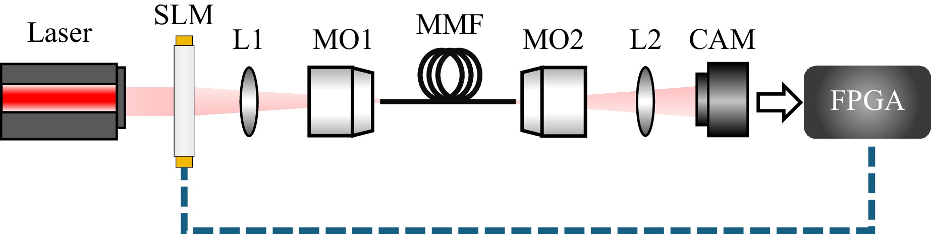
Fig. 5  Scheme of the experimental setup. Abbreviations: CAM, camera; L, lens; MMF, multimode fiber; MO, microscope objective; SLM, spatial light modulator.

As the intensity distribution is originally captured by the camera, the experimental images are processed by square root to obtain the $ U(r,\phi)$. The obtained amplitude images are then cropped to pick up the core region of the MMF. Finally, the cropped image is adjusted to 16 × 16 pixels, and the normalization process is completed to obtain the final input image. For the 100 experimental data images, the Γ between the actual image and the image reconstructed by the CNN model on both the FPGA and PyTorch is 97.07%, and the standard deviation is 0.0219. This demonstrates that the performance of the model is consistent across both platforms. The results regarding the correlation coefficient on 100 experimental data elements are shown in Fig. 6.

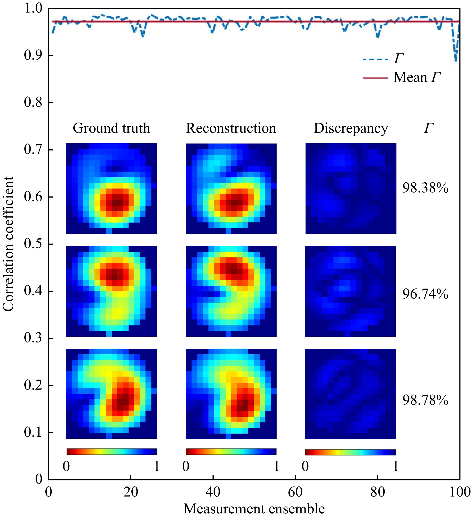
Fig. 6  Test results of MD on experimental data. 3 samples are randomly selected and visualized. The reconstructed, original experimental images (Ground Truth), and their discrepancy are given. The percentage represents the correlation coefficient between the reconstruction and ground truth.

We also investigated the resource utilization and power consumption in FPGA accelerated CNN. Since there are limited DSPs on the FPGA board, optimizing the hardware design needs to be considered to achieve lower power consumption while maintaining consistent performance and running speed. Here, the optimization for the MD for 3 modes has been studied. To optimize resource utilization, data parallelism is first adjusted based on the estimation in the synthesis report in Vivado HLS. These estimates are typically refined during the detailed synthesis and implementation stages in Vivado, which include specific low-level optimizations such as logic sharing, LUT packing, and other architectural considerations. Consequently, after RTL synthesis and implementation in Vivado, the initially high LUT utilization estimates seen in HLS are typically reduced. For this project, the final Vivado report shows that the LUT utilization is set to a reasonable and effective range, as shown in Table 2. The power consumption of different parts is listed in Table 3. The total power consumption in this design is 2.411 Watts, of which 93% is consumed as dynamic power.

The comparison from running the model on FPGA (Zynq 7020 SoC) and GPU (NVIDIA RTX A6000) using the same synthetic data for MD is shown in Table 4. Power is the average power in validation. Efficiency is defined as the number of frames that can be processed per watt. Inference time is defined as how long it takes for one decomposition. Here we show the average result of 100 test data. The table shows that the FPGA requires 5.87 ms to process the prediction for a single decomposition, whereas the GPU takes 2.38 ms. The FPGA’s power consumption is 2.411 Watts, compared to the GPU’s 77.48 Watts, significantly reducing power consumption. The results show that FPGA implementation has higher energy efficiency compared to GPUs (13:1).

We have first demonstrated an FPGA-accelerated deep learning method for demultiplexing the optical signal from MMF based on intensity-only measurement. The neural networks are trained with synthetic data and can work in the experimental environment. The proposed solution shows superior power efficiency compared to the MD using GPUs. At present, we have successfully implemented neural networks into an FPGA for mode identification of up to 30 modes with 100% accuracy and decomposition of 6 modes with a minimal correlation of around 90%. Our method does not need a reference beam in the experimental setup and works in a single-shot way without iteration.

A comparison between the different numbers of modes and the platforms (see Table 1) shows that there is a performance drop with the increasing number of modes. The main reason here is that the complexity of the problem increases exponentially as the number of modes increases. With a limited number of layers and neurons, neural network models cannot make more accurate predictions. Furthermore, compared with the floating-point model in PyTorch, the accuracy of the quantized model on the FPGA on the test data also decreases. The more layers there are, the more obvious this decrease will be. The reason is that the quantized model inevitably produces a certain amount of accuracy loss in each calculation. When the network is deeper, this loss also gradually accumulates. Compared with the performance of the neural networks on synthetic data, the accuracy of the actual data is reduced. This is mainly due to the fact that the optical setup is not perfect and there is some noise in the experimental images. It is possible to label the experimental images using, for example, using DH¹¹ to create datasets for the training. Modeling the noise and adding it to the synthetic data is another possible approach to minimize the performance loss on real data. Additionally, the image processing including the cropping and resizing brings errors to the decomposition. Unlike other deep learning-based MD studies in which the absolute or cosine value of the phase weights is used^4,15,20, we limit the phase range of the second mode to eliminate the phase ambiguity problem. As no post-processing is necessary, our method works much faster. However, CNNs trained with limited phases require more epochs to converge. This could be attributed to the fact that there are fewer cases of phase combinations in the dataset consisting of absolute phase values. Additionally, as the phase range is limited, the predicted phase value might be the conjugation of the optical field. An inversion of the phase sign may be required for realizing pre-distortion to undo the scrambling in MMF communication⁷.

In general, our method can be improved with respect to decomposition accuracy and inference speed. The FGPA used in this work has very limited resources (mainly the number of DSPs and LUTs), which limits the degree of parallelization of computation and the complexity of the neural network. Higher data parallelism and optimization of the pipeline can reduce the inference time. Furthermore, as the fiber has a round core, circular images and circular convolutional kernels³² can be used in the future to reduce memory and computational resources. To increase the accuracy, more advanced neural networks (like MTNet²⁰, and DenseNet⁴) can be implemented. Additionally, in order to maintain the performance of the trained neural networks, quantization plays a crucial role. Advanced quantization methods can benefit from reducing the performance loss. It is worth mentioning that implementing neural networks on FPGAs presents challenges, especially in terms of architecture construction and operational speed. Compared to the more straightforward setup on CPU and GPU platforms, configuring neural networks on FPGAs involves a more complex design process. This complexity stems from the need to manually optimize hardware configurations to suit specific computational tasks, which requires in-depth knowledge of hardware design³³. Consequently, many recent studies focus on mitigating these drawbacks by exploring various optimization strategies³⁴⁻³⁶. These strategies include algorithmic refinement, hardware-software co-design, and the development of specialized tools and frameworks that enhance the performance of neural networks on FPGAs.

Whether deep neural networks run on GPUs or FPGAs is more of a trade-off. FPGA has a unique advantage in closed-loop control since data transfer latency is lower than GPU³⁷, which is crucial in time-sensitive scenarios, like telecommunication. Additionally, FPGAs can perform well when handling data input from multiple sensors³⁸, such as cameras, photon receivers, or other sensors, which shortens the calibration process for fiber communication, or fiber laser and fiber sensing. The solution proposed does not have advantages in the number of modes compared to GPU-based solutions. Additionally, it should be noted that GPU is particularly effective for parallel computation rather than single-data or sequential computation. Therefore, the decomposition time per image increases if it is converted to an online real-time MD³⁹. In contrast, FPGAs are better suited for single-frame decomposition. Furthermore, FPGAs can be used for more than just MD using AI by integrating additional capabilities onto the same chip, which makes them ideal for use in industrial and medical fields.

We are confident that the proposed FPGA-based acceleration of MD provides an efficient and compact solution in fast transmission matrix measurement towards secure data exchange like QKD and physical layer security via MMF¹⁴. A real-time closed-loop control system can be built by incorporating a fast SLM and a high-speed camera. When combined with recent advancements in the multiplexing and characterization of MMFs^20,40,41, holds significant promise for cost-effective spatial-division multiplexing systems for high data rate communication. Additionally, our work can be extended to free space communication and other applications, like imaging and sensing for fast data processing and closed-loop control where latency and cost-efficiency are critical⁴²⁻⁴⁶.

FPGA stands for Field programmable Gate Array, which has three main advantages, flexibility, low latency, and high energy efficiency. In this work, the Xilinx Zynq-7020 SoC FPGA is used. This device is unique in integrating the traditional PL component of an FPGA with the PS including a dual-core ARM Cortex-A9 processor on a single chip. The selected FPGA development tool is Vivado 2019.1, and Vivado HLS is used for IP core generation.

The presented investigation aims to train a neural network that can be run on an FPGA system to accelerate the decomposition process. In this work, CNNs were used to classify the eigenmodes and decompose the distal speckle images. Convolutional layers, the core component of a CNN, are often used to process image data to extract valid information from the image with a convolutional operation and pass it to the next layer³⁰. Each convolution operation involves numerous multiplications and additions, which can be efficiently accelerated using the parallel processing capabilities of an FPGA.

Fig. 1 visualizes the neural network structure for mode classification. This network consists of 3 convolutional layers with downsampling for encoding and 2 fully connected layers for classification. All convolution kernels are 3 × 3, and all max pooling kernels are 2 × 2. The output size of the feature map is denoted below of box. For all the training cases from 3 to 40 modes, the learning rate is set as 0.0001. The cross-entropy loss function and the Adam optimizer are selected. For classification from 3 to 19 modes, the network is trained for 15 epochs with a batch size of 64. For 19 to 40 modes, due to the increasing complexity, the network is trained for 40 epochs with a batch size of 128.

For MD, the complexity of the task is higher due to the presence of an infinite number of mode combinations. As the number of modes increases, the corresponding number of CNN layers also needs to be increased to accommodate the training needs of more modes. In addition, in order to better capture and distinguish the details of different modes, higher resolution images are used, which increase the amount of mode information in the image. These adjustments improve the network’s ability to recognize different patterns, thereby ensuring the accuracy and reliability of the model. Table 5 shows the details of the configuration. To address the 3-mode decomposition, 40,000 pairs of data are generated and divided into the training, validation, and test datasets. The model is trained with a batch size of 256, 1500 epochs, and a learning rate of 0.0006. For 5 and 6 modes, these parameters are adjusted accordingly. Due to the increasing complexity, 100,000 pairs of data are generated. This model is trained with a batch size of 512, 1000 epochs, and a learning rate of 0.001. In all cases, the validation and test dataset has 1000 pairs of data. All the remaining data is used as the training dataset. The MSE loss function and the Adam optimizer are used, as they are suitable for the regression task of MD⁴⁷.

Classification accuracy is used as a metric to evaluate the performance of CNNs in the mode classification, which is calculated as:

To quantify the performance of the MD algorithm, the reconstructed field distributions are compared with the original (target) field distributions, where correlation coefficient (Γ) is used and defined as below:

where $ {I}_{T} $ is the target mode distribution and $ {I}_{R} $ is the reconstructed distribution. $ ROI $ refers to the entire area of interest. Intensity distribution I indicates the mean value of the respective intensity distribution. The value of $ \varGamma $ presents how similar the reconstructed intensity distribution is to the target. The relative error between the predicted mode weights and the target mode weights are introduced as the metric and defined as: $ \text{Δ}\rho =|\sqrt{{{\rho }_{p}^{2}}}-\sqrt{{{\rho }_{t}^{2}}}| $, $ {\Delta }\rho =({|{\phi }_{p}-{\phi }_{t}|})/{2{\text π}} $. Here, “$ p $” indicates a predicted value, and “$ t $” denotes a target value. Additionally, the standard deviation σ is used to evaluate the robustness of the DNN-based MD system. σ is determined as follows: $ \sigma =\sqrt{{1}/({K-1}){\sum }_{k=1}^{K}({{\Gamma }}_{k}-\overline{{\Gamma }})} $.

Quantization is the process of converting values with higher precision, such as floating point numbers, into values with lower precision, such as integers. For FPGAs, quantization reduces model weights, bias, and activations from floating-point numbers (e.g., 32-bit floats) to lower bit widths (e.g., 16-bit integers). This reduction significantly decreases storage requirements, enhances computational speed, and reduces power consumption. By minimizing data bit-widths, larger models or more layers can be run on limited hardware resources, improving hardware utilization⁴⁸. In general, there are two main classes of quantization: static quantization and dynamic quantization. Static quantization is to quantize the weights and activation values of the model before inference. Dynamic quantization is to dynamically adjust the quantization parameters according to the data during the inference process. This increases the complexity and uncertainty of the calculation and is not suitable for FPGA systems that require high certainty. Therefore, in this work, the fixed-point quantization method in the static quantization method is chosen. Fixed-point quantization converts floating-point numbers to integers by multiplying by a fixed scaling factor and then rounding. Fixed-point numbers can represent integers or decimal numbers, depending on the position of the radix point, also known as the Q-value. The Q-value determines the precision and range of the representation. Floating-point numbers have a dynamic radix point position, providing higher precision but a narrower range. In contrast, fixed-point numbers have a fixed radix point position, offering a wider range but lower precision. Using a fixed Q-value, the weights and biases of each layer are quantized, converting them into fixed-point numbers, which can be represented by the following equation:

where $ {x}_{q} $ is the fixed-point number, $ {x}_{f} $ is the floating-point number, and $ Q $ is the radix point position. The conversion back to floating-point is represented as:

While fixed-point quantization simplifies computation and reduces storage requirements by simply converting floating-point numbers to fixed-point numbers, this conversion also introduces truncation errors, leading to accuracy loss. A higher Q-value results in a smaller decimal range and higher precision, while a lower Q-value results in a larger decimal range and lower precision. Hence, a trade-off between decimal range and representation accuracy in fixed-point numbers is required. In the task of mode classification, for the fixed-point quantization of weights, inputs, and activation to 16-bit fixed-point numbers, a Q-value of 10 is chosen, corresponding to a scaling factor of 1024. This choice expands the overall range of representable values while maintaining reasonable decimal precision. In the test case of mode decomposition, a Q-value of 12 is chosen for the 16-bit fixed-point quantization, corresponding to a scaling factor of 4096. The precision in decimal places is calculated as follows:

As a result, the precision is equivalent to approximately 3.01 and 3.61 decimal places for the classification test and decomposition task, respectively. This decision is made by examining the parameter sizes of the exported CNN model and analyzing the distribution of input values and activation values in each layer after testing the model with a large number of input images. This Q-value ensures that the quantized model maintains high accuracy while optimizing resource usage on the FPGA.

This research was funded by the Federal Ministry of Education and Research of Germany with the project 6G- life (grant identification number: 16KISK001K) and QUIET (project identification number: 16KISQ092). Furthermore, this work was partially supported by the German Research Foundation for funding (grant number: CZ 55/42-2).