Thin-film neural networks for optical inverse problem

Optical inverse problems, such as optical metrology and inverse optical design, have always been a hot topic because of their wide applications in science and industry^1–4. For conventional frameworks of the thin-film optical inverse problem, two spaces exist: the parameter space and the data space. All the possible parameters of thin films (e.g., thickness and refractive index as a function of wavelength) form the parameter space, while the optical responses of thin films to different parameters (e.g., reflectance spectra) form the data space. To solve a typical thin-film optical inverse problem, the initial parameters in the parameter space are selected as the starting point, and then the optical responses in the data space are computed by electromagnetic simulations. To determine the direction of updates of the optical response in the simulation, the simulated response is compared with the target response, i.e., the measured spectrum for optical metrology and the desired spectrum for inverse optical design. By conducting several electromagnetic simulations in each direction of the parameter space and comparing the differences between the spectra obtained from these simulations, the parameter changes required to update the optical response can be determined. This process was performed iteratively until the simulated response matched the target response. For simple thin films with a few layers, conventional approaches are effective because of the low-dimensional parameter space and reduced calculations. However, with the rapid increase in the number of layers and parameters, accurate thickness characterization and the design of multilayer thin films become more difficult owing to the high-dimensional parameter space and lengthy calculations. To satisfy the demand for fast and convenient solutions to the optical inverse problem, a new framework to solve this problem is required.

Fundamentally, the optical inverse problem is a parameter optimization process of nanophotonic structures. Recent studies on all-optical neural networks (NNs) have established a correlation between multilayer nanophotonic structures and multilayer NNs by exploiting their structural similarity^5–10, making it possible to optimize the parameters of nanophotonic structures during the learning process based on backpropagation. Therefore, common NN training tasks, such as handwritten digit recognition with the MNIST dataset⁵ and human pose estimation⁷, may be achieved with all-optical NNs at a high precision. In this paper, we introduce the idea of exploiting the structural similarity of all-optical NNs for application to the optical inverse problem. Thin-film NNs (TFNNs) are proposed to optimize and extract all the multilayer thin film parameters during the backpropagation process. As the input of TFNNs, incident light fields with normalized source spectra propagate through every film following the calculation steps in the transfer matrix method. Similar to the weights and activation functions when NNs connect two neural layers, transfer matrices characterize the propagation process of the light fields in TFNNs between two thin-film layers. The outputs of TFNNs are the reflectance and transmittance spectra. The thickness and refractive index of each layer in the thin films become the TFNN parameters. Then, in the new framework, the thickness and refractive index in each layer in the thin films can be optimized through the training process based on backpropagation in TFNNs, which is very similar to the process in NNs.

In this paper, we first explain the principle of the optical inverse problem with the NN-like framework. Mapping from the data space to the parameter space is implied in the training process of TFNNs. Then, the mathematical details of TFNNs are demonstrated by exploiting their structural similarity with multilayer NNs. In the section on optical metrology, the reflectance of thin films at normal incidence is measured as the target for training TFNNs. For monolayer thin films, both the thickness and refractive index of the layer are optimized. The multilayer thin films are treated as TFNNs to optimize all the thickness in hundreds of layers. The time required for optimization is significantly shortened compared with conventional methods (e.g., for thin films with 232 layers, conventional approaches take 67.498 s per iteration; our method takes 0.924 s per iteration). In the section on inverse optical design, the design of multilayer thin films based on TFNNs is introduced. Then, we designed and fabricated three types of multilayer thin films that mimic three types of cone cells in the human retina. An image-forming system is built, which records the light passing through these multilayer thin films as a colored photo.

Fig. 1 shows the parameter space and data space in conventional approaches. A group of thin-film parameters is represented by small spheres in the parameter space, while the spectrum of the thin films is represented by rectangular solids in the data space. Each small sphere corresponds to a rectangular solid through electromagnetic simulations, as shown by the arrows from the parameter space to the data space. For a group of parameters represented by the red sphere, its convergence direction to the minimum point in the parameter space was obtained by additional electromagnetic simulations at the neighboring points denoted by the blue sphere. The number of neighboring points required is proportional to the dimensions of the parameter space.

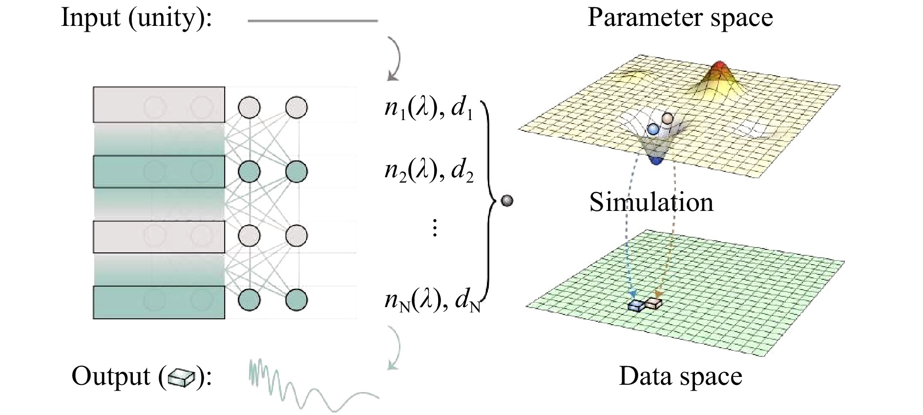
Fig. 1  The framework inspired by all-optical neural networks.

The framework of the solution inspired by all-optical neural networks (left panel) and its correlation with the conventional framework (right panel). For conventional frameworks, to obtain the convergence direction of the red sphere (current parameters), an additional simulation is required at the blue sphere (neighboring parameters) to compare the difference in their spectra, marked as red and blue rectangular solids, respectively. For our new framework in the left panel, the convergence direction was obtained through the backpropagation process of TFNNs during training; hence, no additional simulation is required.

For the new framework inspired by all-optical NNs, the input of TFNNs is a normalized source spectrum, and their output is the reflectance or transmittance spectrum of the thin films, denoted as $ R={\left|r\right|}^{2} $, where $ r $ is the Fresnel reflectance or transmittance. Thus, the spectrum of thin films represented by the rectangular solid in the data space is converted into the output of TFNNs. A group of thin-film parameters represented by a small sphere in the parameter space is converted into the parameters of TFNNs, as shown in Fig. 1. Based on the above analogies, the backpropagation process of TFNNs can be established to obtain the convergence direction of every parameter in one calculation if the structural similarity between thin films and NNs is exploited.

To compare the structure of thin films and NNs, diagrams of multilayer thin films and multilayer NNs are shown in Fig. 2. For thin films, there is an interface between the neighboring layers; for NNs, there is a corresponding weight connection between the neighboring layer of neurons. For thin films, there is a bulk of the layer between the interfaces, whereas for NNs, there is a corresponding layer of neurons between the weight connections. Taking $ i-1 $ and $ i $ layers as an example, the interfaces, bulk, and field amplitudes of each layer in the thin films are plotted on the left panel in Fig. 2. The corresponding weights, neurons, input, and output of each layer in the NNs are plotted on the right panel in Fig. 2. For thin films, $ {a}_{i-1} $ and $ {b}_{i-1} $ represent the field amplitudes on the upward side, and $ {c}_{i} $ and $ {d}_{i} $ represent the field amplitudes on the downward side of the $ i $-th interface. For NNs, $ {\boldsymbol{X}}_{\boldsymbol{i}\bf -1}={\left[{x}_{i-1}^{1},{x}_{i-1}^{2},{x}_{i-1}^{3},{x}_{i-1}^{4}\right]}^{T} $ represents the input and $ {\boldsymbol{Y}}_{\boldsymbol{i}}= $$ {\left[{y}_{i}^{1},{y}_{i}^{2},{y}_{i}^{3},{y}_{i}^{4}\right]}^{T} $ represents the output of the $ i $-th weight connection.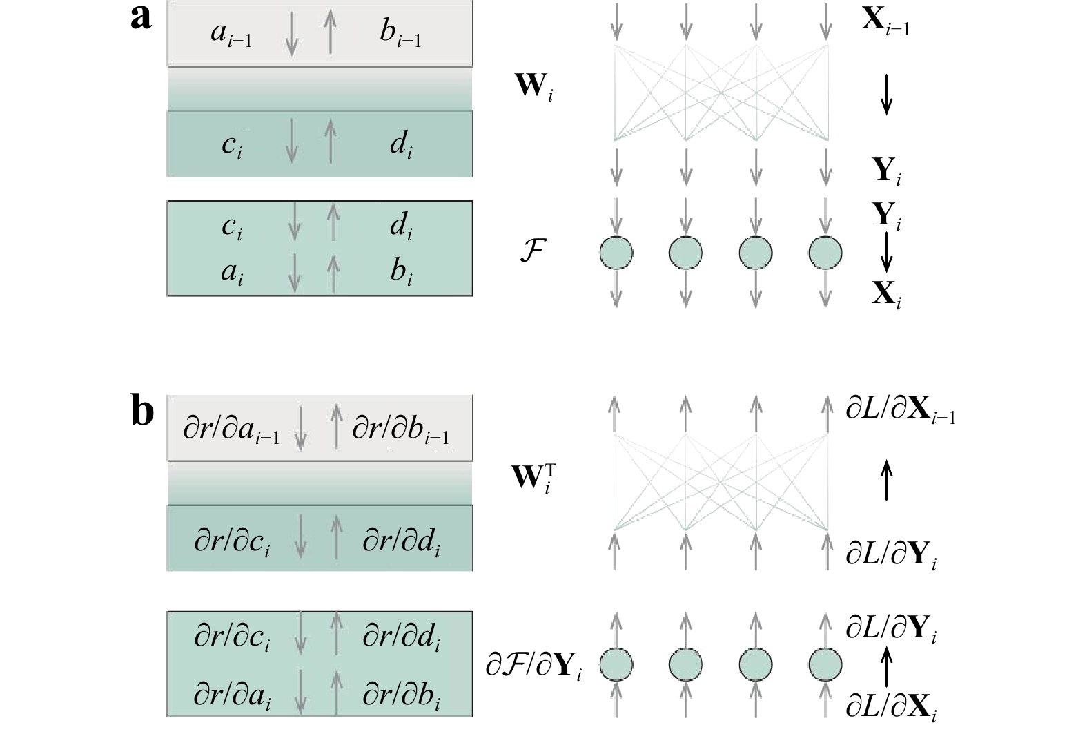

Fig. 2  Structural similarity between thin films and NNs.

a The forward propagation process in multilayer thin films and NNs. b The backpropagation process in multilayer thin films and NNs.

For the forward propagation process of NNs in the weight connection, the input and output of the weight connection is $ {\boldsymbol{X}}_{\boldsymbol{i}\bf -1} $ and $ {\boldsymbol{Y}}_{\boldsymbol{i}} $, respectively, as shown in the upper panel in Fig. 2a. $ {\boldsymbol{Y}}_{\boldsymbol{i}} $ is related to $ {\boldsymbol{X}}_{\boldsymbol{i}\bf -1} $ by the weight matrix $ {\boldsymbol{W}}_{\boldsymbol{i}} $, as shown in Eq. 1a. For the forward propagation process of thin films at the interface, the field amplitudes on the upward side of the interface are $ {a}_{i-1} $ and $ {b}_{i-1} $, while the field amplitudes on the downward side of the interface are $ {c}_{i} $ and $ {d}_{i} $. $ {c}_{i} $ and $ {d}_{i} $ are related to $ {a}_{i-1} $ and $ {b}_{i-1} $ by the interface matrix $ {\boldsymbol{T}}_{\boldsymbol{i}} $, given by the boundary conditions of the electromagnetic field^11,12, as shown in Eq. 1b.

For the forward propagation process of NNs in the layer of neurons, the input and output of neurons is $ {\boldsymbol{Y}}_{\boldsymbol{i}} $ and $ {\boldsymbol{X}}_{\boldsymbol{i}} $, respectively, as shown in the lower panel of Fig. 2a. $ {\boldsymbol{X}}_{\boldsymbol{i}} $ is related to $ {\boldsymbol{Y}}_{\boldsymbol{i}} $ by the activation function. The activation function $ \mathcal{F} $ is executed independently in each neuron, which can be viewed as a diagonal matrix, as shown in Eq. 2a. For the forward propagation process of thin films in the bulk of the layer, the field amplitudes on the upward side of the bulk of the $ i $-th layer are $ {c}_{i} $ and $ {d}_{i} $. On the downward side of the bulk of the $ i $-th layer, the field amplitudes are $ {a}_{i} $ and $ {b}_{i} $. $ {a}_{i} $ and $ {b}_{i} $ are related to $ {c}_{i} $ and $ {d}_{i} $ by the propagation matrix. The propagation matrix is also diagonal^11,12, manipulating the field amplitudes independently, as shown in Eq. 2b.

where $ {\phi }_{i} $ is the phase thickness imposed by the bulk of the $ i $-th layer upon one traversal of light in the propagation matrix.

The above comparison shows that the forward propagation processes of NNs and thin films are similar. By analogy with the backpropagation process of NNs, the backpropagation process of TFNNs can be established the same way, as shown in Fig. 2b. The gradients in the NNs and TFNNs, which propagate in the backpropagation process, were set out from the loss function $ L $ and Fresnel reflectance or transmittance $ r $, respectively. The mean squared error (MSE) is often used as a common loss function $ L $ to evaluate the difference between the output and target. Then, the gradients $ \partial L/\partial {\boldsymbol{X}}_{\boldsymbol{i}} $ in NNs and $ \partial r/\partial {a}_{i} $ in TFNNs can be calculated in turn.

For the backpropagation process of NNs in the layer of neurons, the input and output of the layer of neurons is $ \partial L/\partial {\boldsymbol{X}}_{\boldsymbol{i}} $ and $ \partial L/\partial {\boldsymbol{Y}}_{\boldsymbol{i}} $, respectively, as shown in the lower panel in Fig. 2b. $ \partial L/\partial {\boldsymbol{Y}}_{\boldsymbol{i}} $ is related to $ \partial L/\partial {\boldsymbol{X}}_{\boldsymbol{i}} $ by the derivatives of the activation function $ \partial \mathcal{F}/\partial {\mathit{Y}}_{\mathit{i}} $, as shown in Eq. 3a. For the backpropagation process of TFNNs in the bulk of the layer, the gradients on the downward side of the bulk of $ i $-th layer are $ \partial r/\partial {a}_{i} $ and $ \partial r/\partial {b}_{i} $; the gradients on the upward side are $ \partial r/\partial {c}_{i} $ and $ \partial r/\partial {d}_{i} $. Through chain rules, the gradients on the downward and upward sides are related by the propagation matrix, as shown in Eq. 3b.

For the backpropagation process of NNs in the weight connection, the input and output of the weight connection is $ \partial L/\partial {d}_{i} $ and $ \partial L/\partial {\boldsymbol{X}}_{\boldsymbol{i}\bf -1} $, respectively, as shown in the upper panel in Fig. 2b. Through chain rules, $ \partial L/\partial {\boldsymbol{X}}_{\boldsymbol{i}\bf -1} $ is related to $ \partial L/\partial {\boldsymbol{Y}}_{\boldsymbol{i}} $ by the transposed weight matrix $ {\boldsymbol{W}}_{\boldsymbol{i}}^{\boldsymbol{T}} $, as shown in Eq. 4a. For the backpropagation process of TFNNs at the interface, the gradients on the downward side of an interface are $ \partial r/\partial {c}_{i} $ and $ \partial r/\partial {d}_{i} $, while those on the upward side of an interface are $ \partial r/\partial {a}_{i-1} $ and $ \partial r/\partial {b}_{i-1} $. $ \partial r/\partial {a}_{i-1} $ and $ \partial r/\partial {b}_{i-1} $ are related to $ \partial r/\partial {c}_{i} $ and $ \partial r/\partial {d}_{i} $ by the transposed interface matrix $ {\boldsymbol{T}}_{\boldsymbol{i}}^{\boldsymbol{T}} $, as shown in Eq. 4b.

The details of the backpropagation of TFNNs are provided in the Supplementary Information. Note that TFNNs are complex-valued NNs that are different from conventional NNs.

To experimentally test the performance of TFNNs for monolayer and multilayer thin films, a homegrown software based on the C language was written to implement TFNNs, and a reflectometer at normal incidence was built, as shown in Fig. 3a. Fibers F1 and F2 were used to connect the light source and spectrometer, respectively. The light passing through lens L1 and L2 was focused on the wafer surface. The light passing through lens L3 and L4 was eventually detected by the spectrometer. SiO₂ thin films with a thickness of d on Si substrates were selected as monolayer thin film samples. Cauchy equations were used to model the refractive indices of the SiO₂ thin films. Forouhi–Bloomer dispersion relations^13,14 were used to model the refractive indices of the Si substrates.

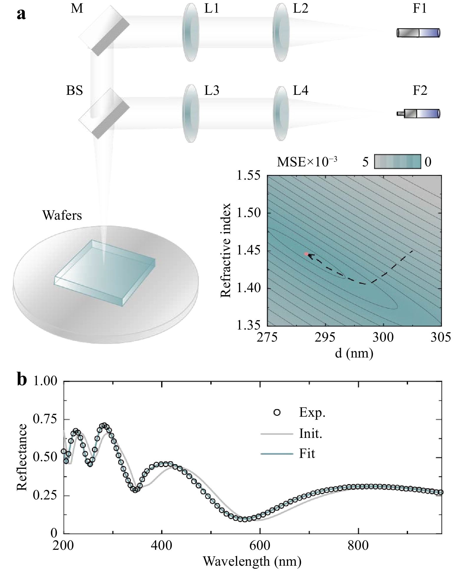
Fig. 3  TFNNs for monolayer thin films.

a Schematic view of the experimental setup consisting of a mirror (M), lens (L), fiber (F), and beam splitter (BS). An example of the parameter space, refractive index, and thickness of SiO₂ thin films on Si substrate, and the convergence process to the minimum points. b The measured, initial, and fitting spectra of SiO₂ thin films on Si substrate.

For monolayer thin films, the training process of TFNNs for extracting the thin-film parameters is shown below. When the measurement was completed, TFNNs take the measured reflectance as the target. The MSE was used to evaluate the difference between the output and target to adaptively adjust the refractive index of SiO₂ thin films and their thickness during the training process. The refractive index of the substrate was fixed. The details of the refractive index of the substrate are presented in the Supplementary Information (S11). Fig. 3a shows the local minimum point in the parameter space. To match the measured spectra, we selected a group of initial parameters as the starting point for the training of TFNNs. The corresponding spectrum of the initial parameters is shown in Fig. 3b (gray line). Then, the gradient direction was obtained by the backpropagation process of TFNNs. Each parameter was adjusted along the gradient direction. At the end of training, the generated spectrum of TFNNs matched the measured spectrum, as shown in Fig. 3b (cyan line). The entire TFNN training process for monolayer thin films (four parameters) was completed in 0.1 s. Additional examples of monolayer thin films with different thicknesses are provided in the Supplementary Information (S9). TFNNs are not only suitable for normal incidence cases but also abnormal ones. Additional examples of abnormal incidence cases are presented in the Supplementary Information (S10).

Next, we turn to multilayer thin films. TFNNs were tested for three types of multilayer thin films with 2, 60, and 232 layers, as shown in Fig. 4. The training process of the monolayer and multilayer thin films is essentially the same; however, only the thickness in each layer was optimized for multilayer thin films. Additional examples on optimizing the thickness and refractive indices of SOI wafers are presented in the Supplementary Information (S12). The thin films with 60 and 232 layers that were set to be periodic at the beginning of the TFNN training became quasi-periodic at the end of training. The initial, fitting, and measured spectra were compared after the TFNN training process, as shown in Fig. 4. For thin films with two layers, the training of TFNNs eliminated the difference between the initial and measured spectra. For thin films with 60 layers, an excellent fitting result was obtained despite the large shift between the initial and measured spectra. For thin films with 232 layers, the spectra of periodic multilayer thin films usually have fringes with greater amplitudes than the measured ones. After the training of TFNNs, the decrease in amplitude made the simulated spectra more consistent with the measured spectra. It is interesting to note that quasi-periodic multilayer thin films usually have larger band gaps than the periodic ones, as shown by the band gaps in the 232-layer films. The optical inverse problem of 3D NAND, i.e., the detection of the erroneous layer in 3D NAND, is shown in the Supplementary Information (S13) as a potential application of TFNNs. A discussion of the further reduction of differences and errors is also provided.

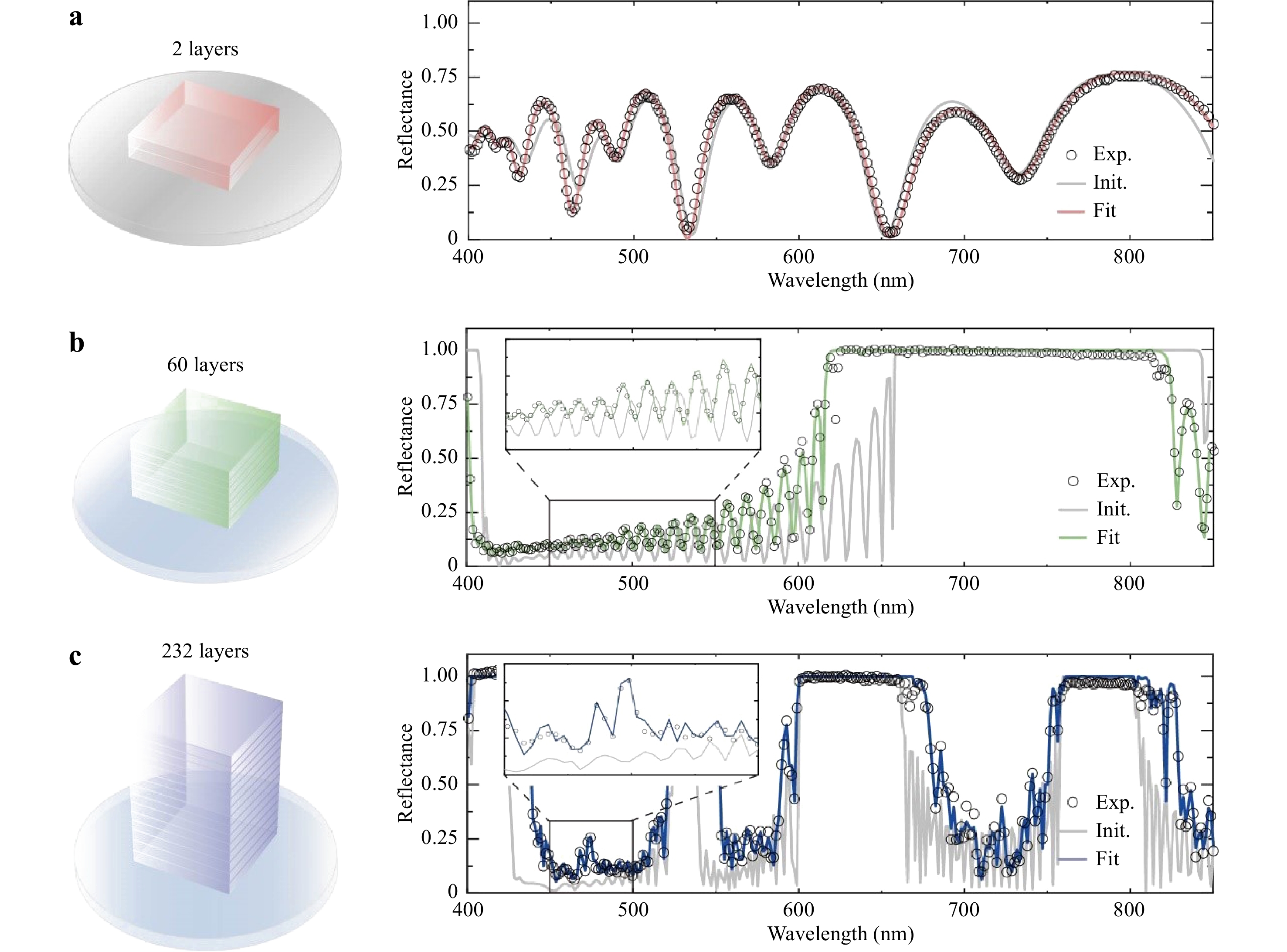
Fig. 4  TFNNs for multilayer thin films.

aThe schematic view of 2-layer thin films (left). The measured, initial, and fitting spectra of 2-layer thin films (right). b The schematic view of 60-layer thin films. The measured, initial, and fitting spectra of 60-layer thin films (right). c The schematic view of 232-layer thin films (left). The measured, initial, and fitting spectra of 232-layer thin films (right).

TFNNs were compared with the conventional framework. The iteration time required in the conventional framework and TFNNs for multilayer thin films with 2, 60, and 232 layers are listed in Table 1. For the conventional framework, the iteration time increased as the number of layers increased. In contrast, the iteration time in TFNNs barely increased with the increase in the number of layers. It should be noted that when the number of layers is less than two, the conventional framework is faster because it requires only one simulation, whereas TFNNs require two complete propagations, i.e., forward propagation and backpropagation. The details of the comparison with the conventional framework are provided in the Supplementary Information (S6).

In this section, another optical inverse problem, i.e., thin-film inverse optical design, is discussed based on the TFNNs. For a particular design task, a large number of adjustable parameters and multilayer thin films can improve the correspondence between the designed and target optical response; however, these also increase the difficulty of fabrication. Thus, the number of layers should be determined according to the maximum tolerable deviation between the designed and target spectra. However, in previous data-driven inverse design methods, changing the number of layers in the model is quite difficult, and often requires training a new model. Because TFNNs are not data-driven and a new layer can be directly added to previous layers, the process is not difficult. Complex thin films with many layers can be easily built on previously trained multilayer thin films with fewer layers. This design process allows us to retain and transfer the information learned during the training of multilayer thin films with fewer layers. When a new layer is added to previously trained multilayer thin films, its role is to reduce the residual (i.e., MSE) between the output and the desired spectra in the new training process, as shown in Fig. 5a. Once the maximum tolerable deviation between the output of TFNNs and the desired spectrum is set, we can determine the number of layers and the thickness of each one. The details of the reuse properties of TFNNs are presented in the Supplementary Information (S14).

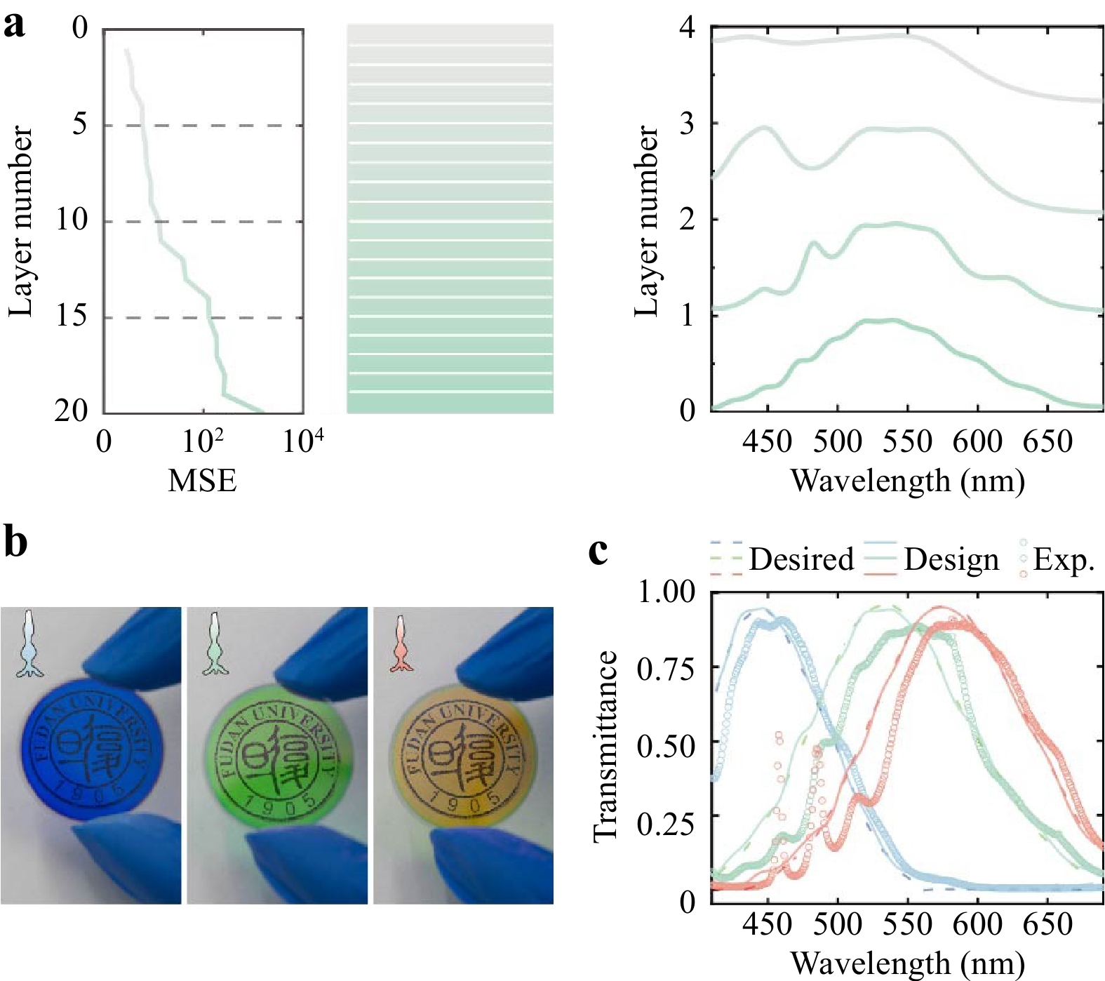
Fig. 5  TFNNs that mimic three types of cone cells in human retina.

a The design idea and process of TFNNs for multilayer thin films. More layers are added to reduce the residual between the output and target spectra, represented by the MSE. b The three fabricated types of multilayer thin films. c The target, designed, and measured spectra of multilayer thin films, whose transmittance spectra are designed to approximate the spectral sensitivity functions of cone cells in the human retina.

To take colored photos, most physical imaging systems, particularly digital cameras, use three different filters to mimic human eyes. However, their sensor responses slightly overlap compared with the spectral sensitivity functions of cone cells in the human retina, which is considered a significant difference¹⁵. With regard to the spectral sensitivity functions of cone cells in the human retina as the goal of inverse design, we used TFNNs to design three types of multilayer thin films to simulate the optical response of cone cells and color perception.

The design process of multilayer thin films for mimicking the spectral sensitivity functions of green cone cells is shown in Fig. 5a. The multilayer thin films consist of alternative SiO₂ and TiO₂ films of differentthicknesses. The MSE decreased with the continuous addition of new layers. When the number of layers reached 20, the MSE between the TFNN output and the target was less than 10^-3, which indicates a good match between the designed and target spectrum. We designed and fabricated multilayer thin films (Fig. 5b), with overlapping spectral sensitivities, particularly those of green and red cone cells (Fig. 5c). We built an image-forming 4F system, in which the light passing through the designed multilayer thin films is recorded as an image in each color channel, as shown in Fig. 6a. Then, a colored photo of a macaw's feathers is produced by superposing the images on all color channels, as shown in Fig. 6b.

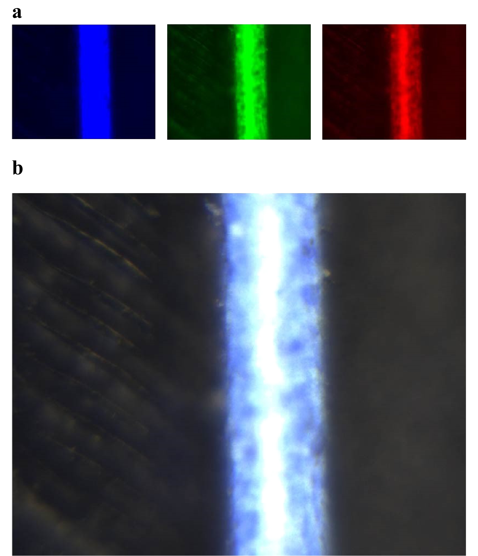
Fig. 6  Color photo of a macaw's feathers obtained using the fabricated multilayer thin films.

a The recorded images on each color channel (blue, green, and red). b The colored photo produced by superposing images on all color channels.

In summary, we proposed the concept of exploiting the structural similarity of all-optical NNs and thin films, and applied it to the optical inverse problem. Thus, we proposed TFNNs as a new framework for the thin-film optical inverse problem. A connection between multilayer thin films and multilayer NNs was constructed by exploiting their structural similarity. In optical metrology, through the training of TFNNs for extracting thin-film parameters, we can effectively optimize all the parameters in monolayer and multilayer thin films. In inverse optical design, we introduced the design idea and process of TFNNs. Then, TFNNs were used to design multilayer thin films to mimic the optical response of three types of cone cells in the human retina.

To obtain a more in-depth understanding of TFNNs, we distinguished our TFNNs from previously reported artificial neural networks (ANNs) for inverse optical design^16–24. For ANNs, the structural parameters and thickness of each layer were used as the input, while the optical responses and spectra of the thin films were used as the output. Then, the ANNs can learn how to approximate Maxwell’s equations. For the training of ANNs, a dataset was required (50,000 samples for thin films with 8 layers¹⁶, and 500,000 samples for thin films with 20 layers¹⁷). The details of using ANNs to solve the optical inverse problem of thin films with hundreds of layers are provided in the Supplementary Information (S7). The input of TFNNs is a normalized source spectrum; the output is the reflectance spectrum of the thin films. Because it is directly constructed using Maxwell’s equations, the spectra generated by TFNNs are accurate. For the training of TFNNs, the parameters can be updated according to the gradient obtained from the backpropagation process of TFNNs, without datasets for thin films with hundreds of layers. The details of the comparison between TFNNs and ANNs are presented in the Supplementary Information (S8).

For the further development of TFNNs, we note that the interface matrix and propagation matrix are all 2 × 2 complex matrices. This indicates that there are only two complex neurons in each layer. To add more neurons in each layer, uniform layers can be replaced by textured layers²⁵. The electromagnetic fields and permittivity function were expanded into a Fourier series to determine the eigensolutions of Maxwell's equations in a periodic textured medium. The eigenmodes interacted with each other at the interface and propagated independently in the bulk of the layer. The size of the interface matrix and propagation matrix was dependent on the order of the Fourier expansion²⁶. The extension of this method to other nanophotonic structures is discussed in the Supplementary Information.

A homegrown program was written in C language to implement TFNNs because of the speed of the C language. The entire framework can be divided into three parts: LinearC, Model, and LMAlgo (details in the Supplementary Information, S15). LinearC provides basic mathematical functions based on the BLAS and LAPACK²⁷. A model was built to construct the forward propagation and backpropagation processes of TFNNs. LMAlgo is the optimal algorithm based on the Levenberg–Marquardt algorithms²⁸ for training TFNNs.

To provide a fair performance comparison, we tested the conventional framework and TFNNs on the same platform: a personal computer with an Intel(R) Core(TM) i5-4210H CPU (2.90GHz). Both the conventional framework and TFNNs used the C language as the backend and Python as the frontend by building C extensions. Note that Python was only selected because of its convenience and universal use. Other frontends, such as C#, can also be constructed for other purposes.

This work was supported by the China National Key Basic Research Program (2018YFA0306201) and the National Science Foundation of China (11774063, 11727811, and 91963212). A.C. was supported by the Shanghai Rising-Star Program (20QR1402200). L.S. was further supported by the Science and Technology Commission of Shanghai Municipality (19XD143600, 2019SHZDZX01, 19DZ2253000, 20501110500).