Melt pool monitoring in laser beam melting with two-wavelength holographic imaging

Additive manufacturing (AM) is a key technology that allows building structures by the progressive addition of materials with complex geometries that cannot be achieved with conventional machining techniques. For example, complex honeycomb structures, called “lattices”, can be realized through topological optimization. AM represents a unique opportunity to optimize and lighten structures and thus reduce energy consumption. Metal additive manufacturing processes, mainly used in the aerospace, energy, automotive, and medical sectors, are categorized into two main families: powder bed processes (LBM: laser beam melting; SLM: selective laser melting; EBM: electron beam melting; and MBJ: metal binder jetting) and directed energy deposition processes (WAAM: wire-arc additive manufacturing; EBAM: electron beam additive manufacturing; and LENS: 3D metal printing by laser deposition and fusion). Mass production of customized structures can be realized with AM. This property is particularly interesting for art and design, but also for medicine and dentistry: prostheses or implants can be adapted to each patient.

In the LBM process, metal or ceramic powder layers are successively melted to manufacture 3D mechanical parts¹. A CAD model of the object to be built is created from a dedicated 3D modeling software and then sliced. In the case of metal parts, LBM is mainly carried out by melting a bed of metal powder using a high-power laser. First, a thin layer of powders is deposited on a substrate plate, and a very powerful laser (few hundred watts) melts the fine metal powders ($\backsimeq $ 40-60 microns in diameter) following the pattern determined by the computer. A roller (the re-coater) then applies a new layer of powder. The laser draws the next layer. These steps are repeatedly applied until the object is completely realized. The structure is thus built by the successive melting of powder layers.

Owing to the complex physical phenomena involved in the laser-matter interaction, melt-pool morphology instabilities can affect the final quality of the structure and remain challenging to foresee by simulation. Everton et al². listed defects that may occur during the process: pores (gas), balling, inflated powder, and cracks. Sames et al³. identified the same defects and delved deeper, compared to Everton et al., into the relationships between process inputs and defects. Grasso and Colosimo⁴ proposed the classification of defects into six categories: porosity, balling, geometric defects, surface defects, residual stresses/cracks/debonding, and microstructure inhomogeneity.

The lack of repeatability and stability of the process slows the democratization of AM in industry. An AM cycle may take several hours or days. For example, an unacceptable defect that appears in the first few minutes of the cycle means wasting the investment in raw material, energy, and time to produce a non-standard part. Therefore, in situ monitoring and quality control are key issues in the development of AM. X-ray tomography is undoubtedly the most successful of the existing monitoring techniques for metal parts⁵. However, this is an ex situ technique that requires specific facilities. Therefore, to achieve the performance and safety requirements of the aerospace industry, significant efforts have been made over the last ten years to develop monitoring techniques that can be implemented in AM machines and take advantage of the ability to monitor and control manufacturing layer by layer. Several monitoring approaches based on the melt-pool process radiation or with a secondary illumination source have been developed to measure diverse dimensions: length, width, height, and area⁶⁻¹⁶. However, these methods cannot measure the 3D shape (called topography) of the melt pool. Nonetheless, the final track morphology is influenced by volumetric and capillary forces applied to the melt pool^{13, 17}. Therefore, the shape of the melt-pool surface is of primary interest for monitoring its stability. Because of its intrinsic heterogeneity, its movement over the powder bed, and its own dynamics, the measurement of the melt-pool surface shape requires a single-shot full-field acquisition with a short exposure time of a few microseconds. Indeed, the traveling of the processing laser can reach 1 m·s⁻¹ in industrial processes. In this paper, the term full-field means that the image of the area under interest is obtained with no requirement concerning surface scanning. This reveals the ability of the optical setup to yield a collection of data points organized as a fine mesh of the inspected area.

Among the optical approaches for surface shape measurement, two-wavelength digital holography proved to be a relevant tool for desensitized testing. Examples include steep optical surfaces (aspheric mirrors and lenses)¹⁸, large deformation of structures¹⁹, and surface shape profiling²⁰. Such an approach can also be used for surface roughness measurement when the roughness is large compared to the wavelength²¹. A wide range of applications of multi-wavelength holography have also been demonstrated, such as endoscopic imaging^22,23, investigation of mechanical structures²⁴, erosion measurements²⁵, and in-line industrial inspection²⁶. Regarding off-axis digital holography and spatial multiplexing of two-wavelength digital holograms, the operation becomes real-time, in the sense that the surface shape can be measured at each instant at which the holograms are recorded. In this paper, the term real-time refers to the ability of the measurement system to record useful data of the phenomenon of interest at its own temporal scale. It follows that the camera frame rate must be in the range of several thousand Hertz.

In this paper, we propose multi-wavelength digital holography as a proof of concept for in situ investigation of the melt pool during metal additive manufacturing. The paper is organized as follows. First, the principles of digital image-plane holography are discussed. Then, the experimental setup employed in this study is detailed. Finally, we present experimental results. Several experiments were conducted: static tracks, moving tracks, and melt pool without and with powder. A discussion on the experimental results concludes the paper.

Digital holography was experimentally established in the 90’s²⁷⁻²⁹. Recently, many fascinating possibilities have been demonstrated: the focus can be chosen freely³⁰, a single hologram can provide amplitude-contrast and phase-contrast microscopic imaging³¹, image aberrations can be compensated³², properties of materials can be investigated³³, and digital color holography^{28, 34} and time averaging are also possible³⁵. Digital holography can be realized through various architectures such as Fresnel holography, Fourier holography, lens-less Fourier holography, and image-plane holography^{36, 37}. Although these architectures present differences in their implementation, they exhibit the same spatial frequency bandwidth when arranged according to an off-axis approach. In this study, we analyzed a case in which off-axis digital image-plane holograms were recorded. This choice is the most suitable for LBM diagnostics. Indeed, recording a single hologram per instant constitutes a powerful tool for studying dynamic events and carrying out high-speed acquisition. In case of image-plane holography, an imaging system is associated with a variable aperture to produce an image of the scene of interest as close as possible to the sensor area (object projected onto the sensor plane). Note that a slight defocus could be also of interest. At the sensor plane, the reference wave $ \mathcal{R} $ is mixed with the wave from the imaging system $ \mathcal{A'} $ to produce the digital hologram, expressed as

The term $ \mathcal{R}^*\mathcal{A'} $ usually refers to the $ +1 $ order of the hologram, whereas $ \mathcal{R}\mathcal{A'}^* $ refers to the $ -1 $ order. In the off-axis configuration, the reference wave is inclined and impacts the sensor at a certain incidence angle such that its complex-valued amplitude can be written as follows ($ a_R $ is considered a constant and $ (u_0,v_0) $ denotes spatial frequencies):

The recovery of the complex-valued amplitude of the image of the object is obtained by filtering the $ +1 $ order in the Fourier spectrum of the hologram. Filtering can thus be written as follows ($ FT $ means Fourier transform):

Eq. 3 is a convolution formula, and the transfer function $ G $ is given by the bandwidth-limited angular-spectrum transfer function in the Fresnel approximation:

In Eq. 4, $ \lambda $ is the wavelength of light, $ R_u $ is the cut-off spatial frequency of the imaging system, and $ d_r $ is the refocus distance when the projected image is not perfectly focused at the sensor plane. Note that if the image is perfectly in-focus, then $ d_r = 0 $ and the transfer function $ G $ is simply a binary filter centered at spatial frequency $ (u_0,v_0) $ with bandwidth related to $ R_u $. The main parameter of interest in the extracted $ +1 $ order is the optical phase, $ \psi $, which can be used for metrology purposes, such as surface height measurements.

Two-wavelength digital holography has many advantages over single-wavelength holography. With a unique wavelength, the measured surface height is ambiguous when it is larger than the wavelength. Given that the surface of the object is also rough, the surface shape cannot be reconstructed because the phase is extracted from the filtering results from a speckle pattern. Thus, the ambiguity and randomness of the phase can be mitigated by using a second wavelength, leading to the so-called synthetic wavelength. Consequently, the ambiguity is bypassed and the measurement range is increased from microns to millimeters (or larger). With two wavelengths, namely $ \lambda_1 $ and $ \lambda_2 $, the synthetic wavelength is given by $ \Lambda = \lambda_1 \lambda_2/|\lambda_1 -\lambda_2| $³⁸. The surface height of the object, $ h(x,y) $, is calculated using the following equation (here, the illumination and observation of the surface are at normal incidence):

where ($ \psi_1 $,$ \psi_2 $) denotes the optical phases extracted from the two holograms at the two wavelengths.

To obtain real-time measurements of the surface height at the melt-pool area, the simultaneous recording of the two phases ($ \psi_1,\psi_2 $) is required ($ f_{ex} $ and $ f_{ey} $ refer to the spatial sampling frequencies of the sensor, i.e., $ f_{ex} = 1/p_x $ and $ f_{ey} = 1/p_y $, where $ p_x $ and $ p_y $ are the sampling pitches of the sensor). This can be achieved by spatial multiplexing of the two holograms at the two wavelengths, so that a single hologram is recorded for both wavelengths. At the sensor plane, the hologram at $ \lambda_2 $ is recorded simultaneously with that at $ \lambda_1 $, and the spatial frequencies of its reference wave are adjusted so that its $ +1 $ order is localized in the Fourier spectrum, separately from the $ +1 $ order at $ \lambda_1 $. Fig. 1 illustrates the spectral distribution in the Fourier spectrum of spatially multiplexed digital holograms at the two wavelengths. The basic arrangement for producing spatially multiplexed digital holograms is shown in Fig. 2. The two reference beams are inclined with different incidence angles to produce the spatial frequencies ($ u_1,v_1 $) for $ \lambda_1 $ and ($ u_2,v_2 $) for $ \lambda_2 $.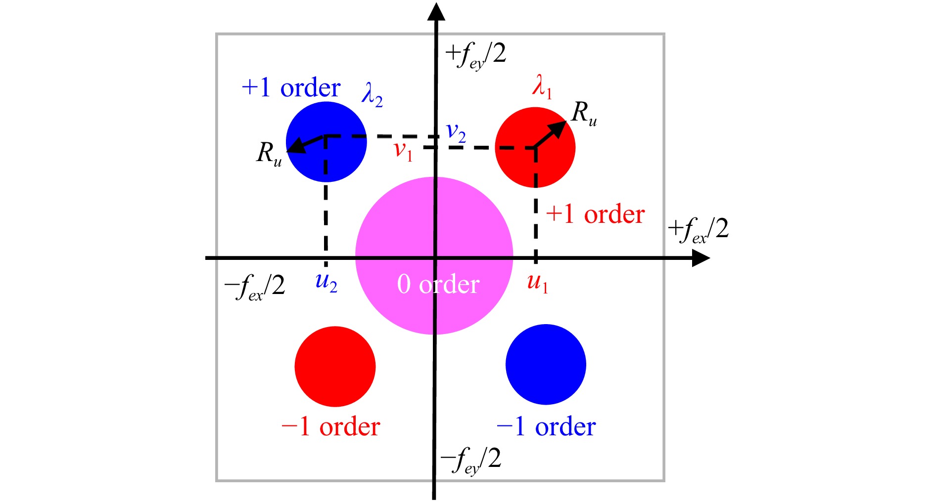

Fig. 1  Spectral distribution of the multiplexed off-axis digital holograms in the Fourier domain at two wavelengths.

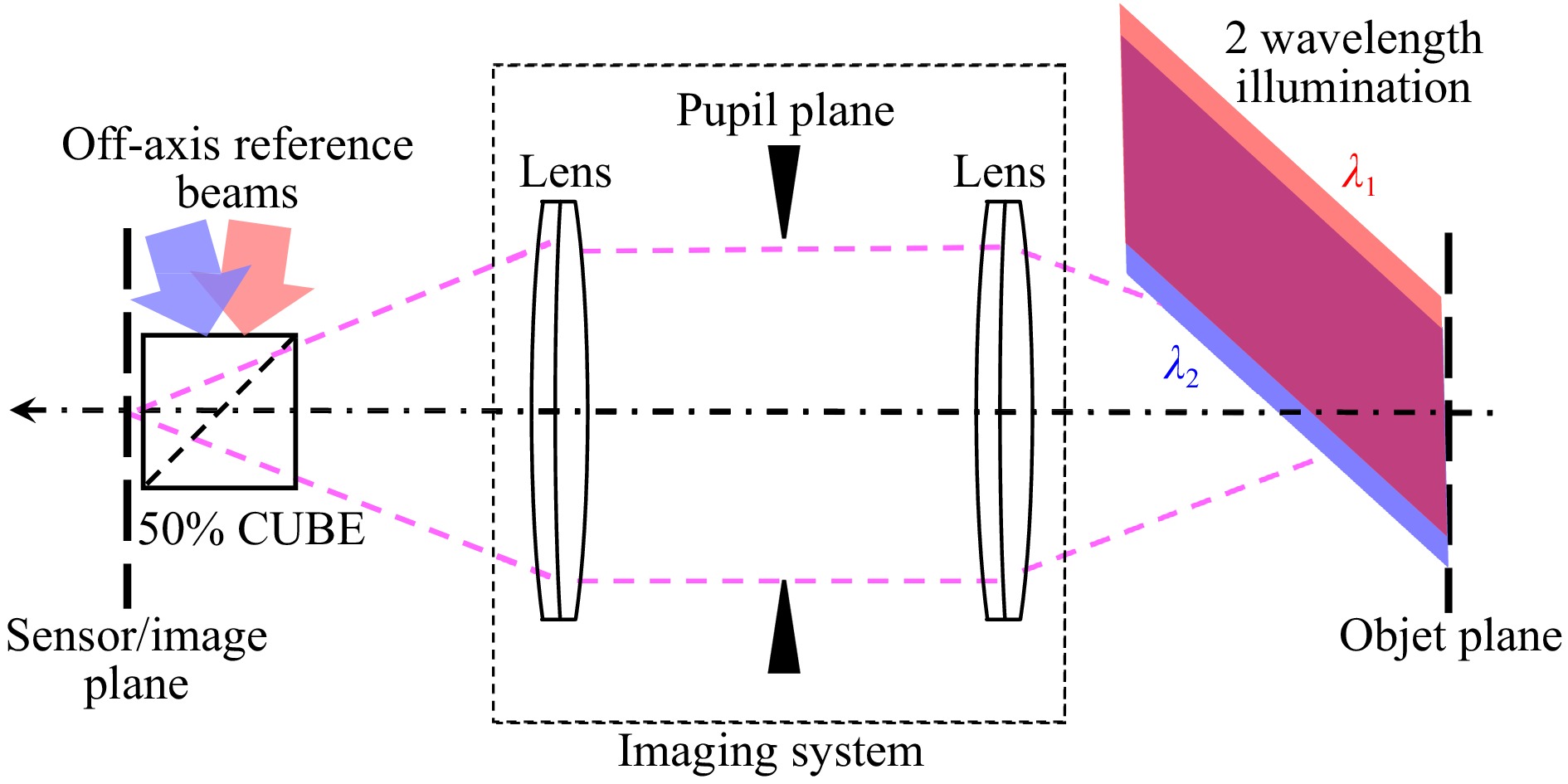
Fig. 2  Imaging of the object area through the image-plane holographic system with spatial multiplexing of the two holograms at two wavelengths.

From a computational point of view, the phase difference expressed in Eq. 5 is obtained by calculating $ \Delta \psi = \arg[C_{12}] = \arg[{A'}_{r2}{A'}_{r1}^*] $, where $ {A'}_{r1} $ and $ {A'}_{r2} $ are the two image fields from the two wavelengths. According to Eq. (3), each of the recovered complex-valued $ A'_{r1-2} $ image includes a bias due to each spatial carrier frequency. More specifically, this bias is due to the presence of the term $ \mathcal{R}^* $ in the output of the Fourier filtering, which must be compensated. This point is discussed in the next subsection.

The compensation of the bias in the phase difference requires knowing the spatial frequencies of the two wavelengths, i.e., ($ u_1,v_1 $) and ($ u_2,v_2 $). These couples can be estimated with spectral analysis when evaluating the centroids of the two $ +1 $ orders in the hologram spectrum (refer to Fig. 1). This yields approximate values that can be used to start the compensation procedure. The method proposed in this paper is to partially compensate for the two carrier frequencies and then refine their residue by using a power spectrum density (PSD) analysis. Thus, partial compensation retains a portion of the frequencies in the complex data $ C_{12} $. The ratio of the spatial frequencies is denoted by $ \alpha $ (typ. $ \alpha = 0.5 $). The partially compensated complex-valued data $ C_p $ can be calculated using the following expression:

PSD analysis is carried out with data $ C_p $ by independently calculating the average PSD along each line and column. Then, the peak in each PSD is detected, and its associated spatial frequency is estimated. For accurate peak estimation, zero-padding of the lines and columns is applied up to $ 2^{16} $ data points. These two estimations over lines and columns yield $ (\Delta u,\Delta v) $. Finally, the residue is compensated according to the expression $ C = C_p \exp(-2 i \pi (\Delta u x+\Delta v y)) $, and the bias-free phase difference is obtained from $ \Delta \psi = \arg[C] = \arg[\mathcal{A'}_{2}\mathcal{A'}_{1}^*] $. This compensation is systematically applied to digital holograms. The next section elaborates on the experimental setup.

The optical setup used to perform topographic measurements on a melt pool is shown in Fig. 3. This includes two modules. In the first module, the holographic module (Fig. 3a), is equipped with two linearly polarized lasers: a 20 mW He-Ne laser and a 50 mW CrystaLaser CRL-DL635-050-SO-Optical-Isolator laser diode characterized by a coherence length of 10 m. These sources respectively emit at 632.8 nm and 634.4 nm, thus yielding a synthetic wavelength equal to 286.74 µm. Both laser beams are expanded before crossing polarizing beam splitters (PBS1 and PBS2). The transmitted beams generate two reference beams, while the reflected beams are superimposed to form a unique probe beam with cube C1 and mirror M3. The probe beam is shaped through beam expander BE3, PBS3, and lens L1, whose focal length is equal to 300 mm, to produce an illumination spot between 0.5 mm and 1mm in diameter. This large illumination allows the exploration of the melt pool and the surrounding area, which is still hot. The quarter wave plate (QWP) between PBS3 and M7 modifies the linear s-polarization into a circular one. The probe beam impacts the surface of interest at normal incidence. After retro-diffusion at the object plane, the QWP modifies the circular polarization of the probe beam into a p-polarization and crosses PBS3 to be directed towards the imaging system composed of the $ 2f_1-2f_2 $ telecentric system and a magnification adjustable as $ G_t = 2 $ and $ G_t = 4.29 $. This system includes a circular pupil with a 20-mm diameter to set the spatial frequency bandwidth $ R_u $ of the holograms. Thus, the imaging system operates with $ R_u = \; 27 $ mm⁻¹. Such aperture is compatible with those commonly used in galvanometer scan heads employed in AM machines (typ. $ f\# 15 $).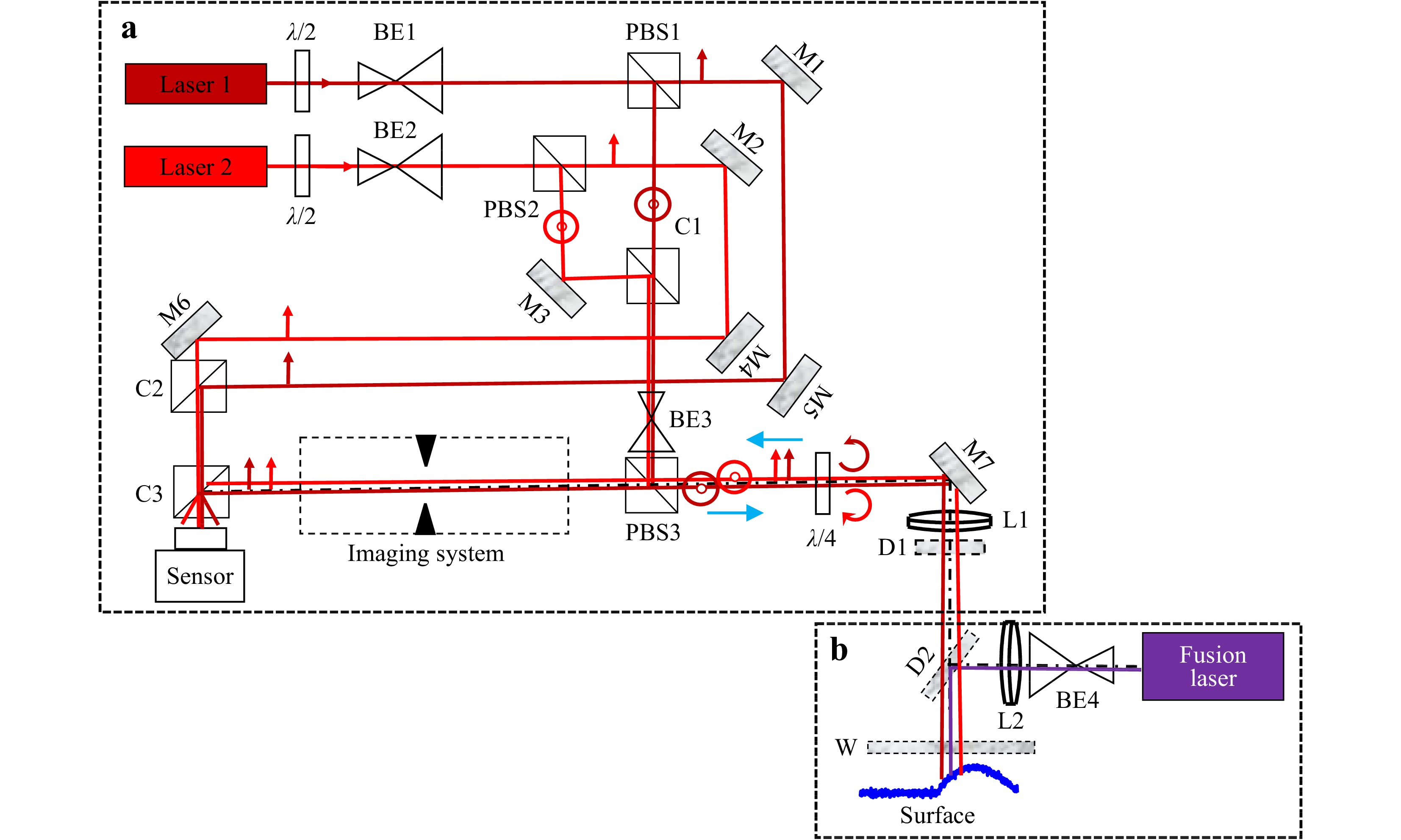

Fig. 3  a Two-wavelength holographic setup for LBM monitoring, b laser fabrication machine (BE1-3: beam expanders, PBS1-3: polarizing beam splitters, M1-7: mirrors, C1-3: beam splitter cubes, D1: chromatic filter, D2: dichroic plates, W: protection window, L1-2: lenses).

The probe beam is mixed with the reference beams at the sensor plane using cube C3. The two reference beams pass through C3, whereas the two probe beams are reflected by C3 to the sensor area. Along the reference paths²⁹, the light impacts the sensor with a slight tilt angle to provide off-axis recording of the holograms. The two reference beams are combined using a splitter cube C2. At the image plane, an 8-bit Photron Fastcam MC2 (pixel pitch of 10 µm) is used to record sequences of two-wavelength digital holograms. The digital holographic system is coupled to a simplified LBM machine, as depicted in Fig. 3b. The two modules are coupled through the dichroic plate D2 characterized by a 980-nm cut-off wavelength so that the light from the processing laser cannot be transmitted to the imaging system. The processing laser is a continuous monomode laser with power adjustable from 50 W to 500 W (SPI laser SM-S00472-8) emitting at 1080 nm and equipped at the end of the fiber with a QBH connector associated with a collimator. The laser power can be adjusted from 50 W to 500 W. The processing laser is equipped with a low-power coaxial laser emitting at 632.8 nm (not shown in Fig. 3b). This alignment laser allows checking that the probe beam and the processing laser are properly superimposed on the powder bed plane. The beam expander BE4 and focusing lens L2 produce, after reflection on the dichroic plate D2 with a cut-off wavelength of 980 nm in the melting zone, a spot whose diameter ranges from 70 µm to 200 µm. The object to be analyzed is installed on a motorized XY stage that permits the alignment and scanning of the processing laser. Note that the dichroic plate D2 operates the first filtering of the thermal radiation from the melting area, while a narrow filter D1 (10 nm) centered around 633 nm drastically reduces this noise source. As a result, a very weak flux of thermal photons may illuminate the sensor. In addition, the light flux from the heated powder bed due to laser fusion is incoherent and cannot interfere with the probe beams. Thus, it is naturally filtered in off-axis digital holography because it is localized in the zero-order lobe (Fig. 1). Nevertheless, the minimization of its contribution at an acceptable level is strategic to avoid image saturation or loss of fringe contrast, which would destroy the useful information contained in the +1 order. The light back-scattered towards the sensor by the processing laser is also filtered by the same optical devices and procedure. Information contained in the zero-order lobe could be exploited to monitor other process signatures, but this is not the purpose of this study. Note that the analysis of the standard deviation of noise in surface-shape data from two-wavelength spatially-multiplexed digital holograms was discussed in³⁹. The influence of noise in the measurements of the surface shape was described using an analytical approach. For further details, please refer to³⁹.

The distance between the powder bed and the last lens in an additive manufacturing machine (DFM system or F-$ \theta $ lens) is generally large because the optics must be protected from spatters or vapor plumes resulting from laser processing. An optical window is inserted to ensure protection. The typical working distances range from 100 mm to 300 mm. Considering that the melt-pool dimensions in LBM processes typically span between 250 µm and 500 µm, the spatial resolution of the holographic system is a key element for defect diagnosis. The circular aperture inserted in the imaging system (refer to Fig. 3a) plays the role of the aperture diaphragm. Thus, this diaphragm is located in the Fourier plane of the imaging system. Its diameter is adjusted to ensure the non-overlap of the diffraction orders in the hologram spectrum (refer to Fig. 2). In addition, it controls the size of the speckle grain in the image plane. As mentioned previously, the aperture is equivalent to a binary spatial frequency filter with a cut-off frequency of $ R_u $. It was demonstrated that the lateral resolution in the object plane $ \rho_x $ of a coherent imaging system is given by $ \rho_x \simeq 0.82 /R_u / G_t $⁴⁰, where $ G_t $ is the magnification between the object and the image plane. Consequently, the average size of the speckle gain at the object plane is equal to $ \rho_x $. With $ R_u \simeq 27\; mm^{-1} $ and $ G_t = 2 $ for a wavelength of 632.8 nm in the holographic system, the spatial resolution of the probe module is $ \rho_x \simeq 15.2 $ µm. This is equivalent to $ f\# \simeq 15 $. Given that the shape of a typical melt pool is characterized by low spatial frequencies⁴¹, approximately ten sampling points should be sufficient to detect defects and classify them.

To qualitatively appraise the quality of the topographic measurement in real conditions, two parallel aluminum alloy tracks realized with the LBM machine were considered. These are remarkably steady experimental conditions because the manufactured object was static, and its structure was stable after cooling. The hologram was acquired with an exposure time $ \tau $ = 145 µs, and the optical magnification was $ G_t = 2 $. From the spatially multiplexed digital hologram, the complex-valued amplitudes for both wavelengths were extracted, and the phase difference was obtained. With the moduli of the complex amplitudes, the autocorrelation of the speckle field was performed to estimate the spatial resolution in the image plane. Fig. 4a shows the autocorrelation function of the speckle field for wavelength $ \lambda_1 $, and Fig. 4b shows its profile along the horizontal line. Note that the autocorrelation function has a width of $ 0.017 $ mm, thus confirming that the spatial resolution in the object plane is approximately 15-17µm, which is in good agreement with the theoretical estimation.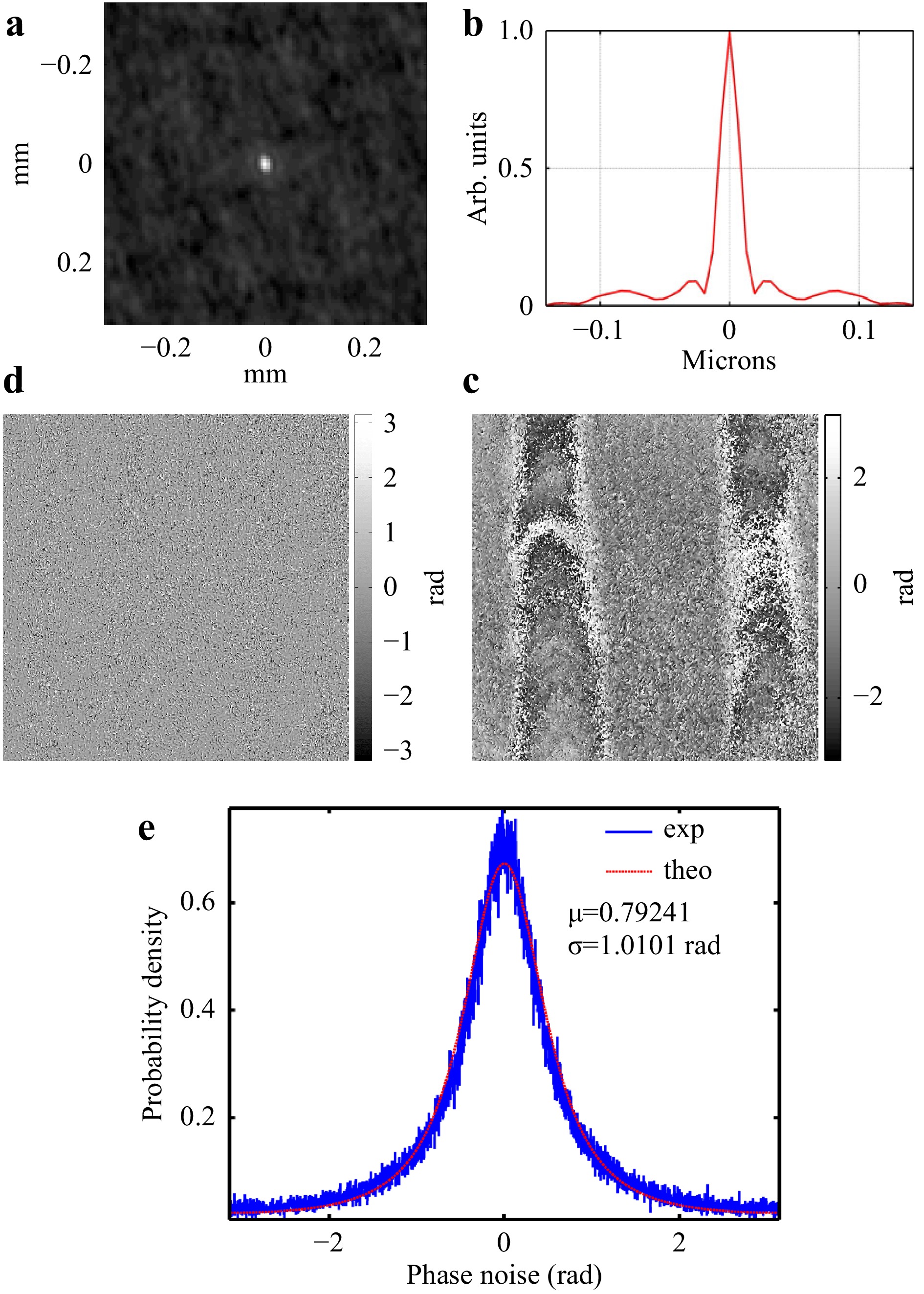

Fig. 4  a Autocorrelation function of the speckle field at wavelength $ \lambda_1 $; b horizontal profile of a; c raw Doppler phase map extracted from the phases at $ \lambda_1 $ and $ \lambda_2 $; d noise map from c; e probability density functions of the phase noise from d (blue line: experiments, red line: theory).

Owing to the surface roughness at the object plane, the phases and the Doppler phase (difference between the two phases $ \psi_1 $ and $ \psi_2 $) extracted from the holograms became corrupted by speckle decorrelation noise. This phase noise can be estimated using a noise estimator⁴². Fig. 4c shows the raw phase map for the aluminum tracks, and Fig. 4d depicts the noise map estimated from the raw Doppler phase. The phase noise is in the range $ [-\pi,+\pi] $ and exhibits non-Gaussian statistics. Fig. 4e shows the probability density functions (PDFs) calculated from the noise map in Fig. 4d. By fitting the experimental PDF with L2-norm minimization, the value of $ |\boldsymbol{\mu}| $ can be estimated from the theoretical equation by using the following relation⁴³⁻⁴⁸ (with $ \epsilon $ denoting the phase noise induced by the decorrelation noise and $ \beta = |\boldsymbol{\mu}| \cos (\epsilon) $):

The coherence factor is a quality metric that indicates the reliability of the phase estimation. Vry et al. ⁴⁹ considered that the standard deviation $ \sigma_{\epsilon} \leq \pi/4 $ is the criterion required for high-quality measurement of the Doppler phase, which leads to the condition $ |\boldsymbol{\mu}| \ge 0.85 $. For other authors⁵⁰, $ |\boldsymbol{\mu}| $ should be higher than 0.37, which is more tolerant to noise but requires a powerful filtering algorithm. In Fig. 4d, the noise standard deviation was found to be $ \sigma_{\epsilon} \simeq 1.01 $ rad $ = \pi/3.11 $, whereas the modulus of the coherence factor was estimated to be $ |\boldsymbol{\mu}| \simeq 0.79 $. Thus, with $ |\boldsymbol{\mu}| \simeq 0.79 $, the measurement can be considered to be of correct quality for the experimental parameters.

Fig. 5 shows the experimental results concerning the topography of the two aluminum tracks obtained with the holographic setup. Fig. 5a displays a photograph of the top-view of the aluminum tracks, and Fig. 5b, c show the topography of the tracks. In Fig. 5d, the region of the tracks represented by the dashed black line in Fig. 5c corresponding to the dashed white line in Fig. 5a, b, is zoomed.

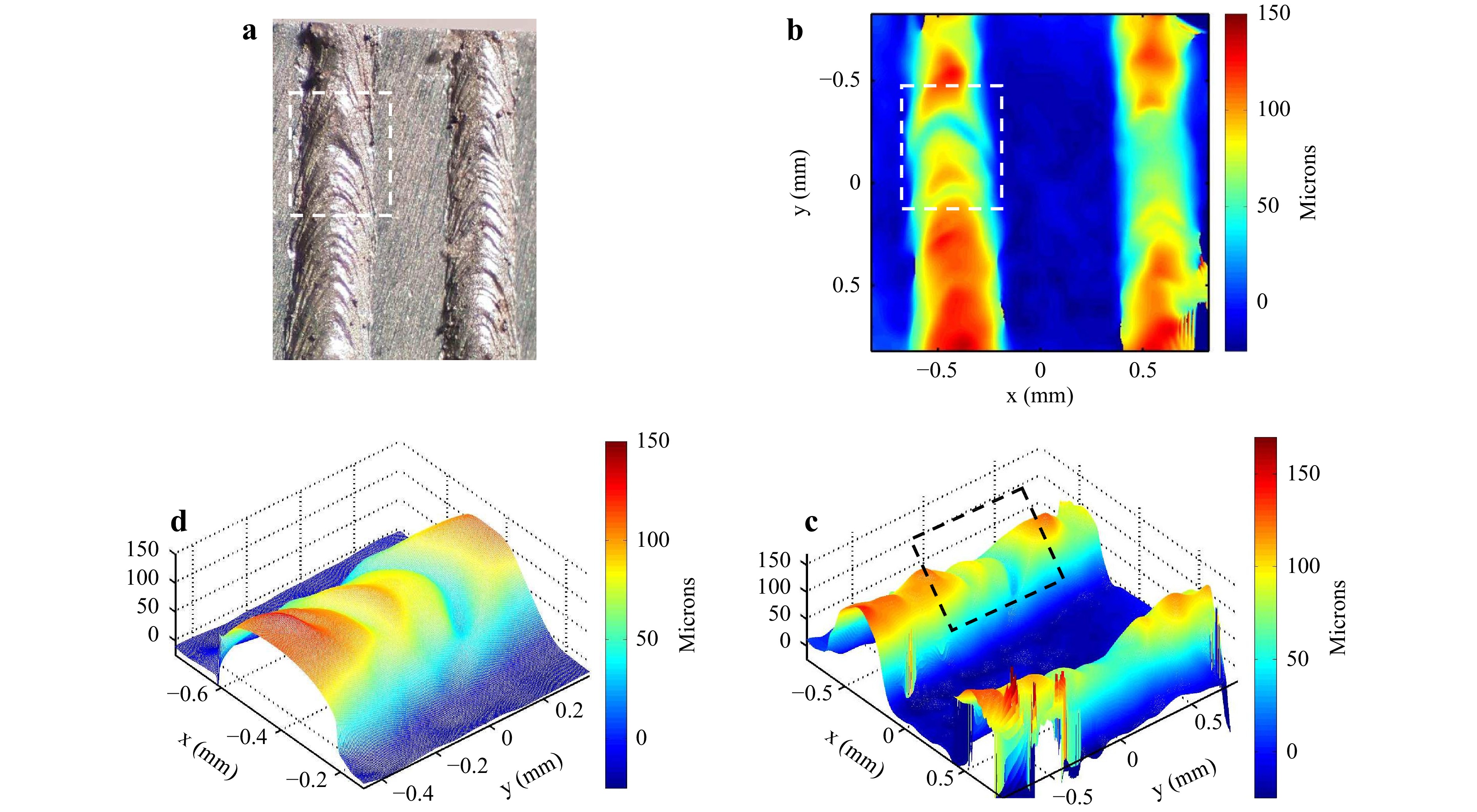
Fig. 5  a Photograph of the top-view of the aluminum tracks for testing the topography measurement; b topography of tracks measured with the setup; c 3D view of b; d zoom of the topography within the dashed black line in c corresponding to the dashed white line in a and b.

When carrying out measurements during the additive manufacturing process, the effect of motion blur on the image quality has to be investigated. This effect is observed along the length of the tracks, which is parallel to the displacement of the motorized stage. If $ V_0 $ is the velocity of the scan at the melt pool and $ B $ is the blur effect expressed as a fraction of the spatial resolution, then we have the following expression:

Motion blur is problematic if $ B $ is close to or larger than one during exposure time $ \tau $. Considering an exposure time $ \tau $ = 25 µs and a spatial resolution of 15 µm, then for $ B = 0.2 $, the maximum allowed scan velocity is 150 mm·s⁻¹. For higher velocities, the exposure time must be reduced according to Eq. 8. For $ V_0 $ = 1 m·s⁻¹, $ \tau $ should not exceed 3 µs. In this case, the monitoring laser power must be sufficient to reach an adequate level of the signal-to-noise ratio of the measurement. To qualitatively check the quality of the measurement for various velocities of the scan, different velocities were set: 100 mm·s⁻¹, 250 mm·s⁻¹, and 380 mm·s⁻¹. For $ V_0 = 380 $ mm·s⁻¹ and $ \tau $ = 25 µs, we obtain $ B = 0.63 $; and for $ V_0 = 250 $ mm·s⁻¹ and $ \tau $ = 25 µs, we obtain $ B = 0.41 $. These values of $ B $ were slightly beyond the limit estimated using Eq. 8. However, for $ V_0 = $$ 100 $ mm·s⁻¹ and $ \tau $ = 25 µs, we have $ B = 0.16 $, which is reasonable. When processing the digital holograms for the three velocities, the values of $ |\boldsymbol{\mu}| $ were systematically estimated to check the overall quality of the holographic measurements in terms of phase noise. For each experiment, the values of $ |\boldsymbol{\mu}| $ remained higher than 0.85, which means that for this set of velocities, the noise quality criterion was respected. However, this criterion did not prevent the measurement from presenting other artifacts such as motion blur. Fig. 6 shows the manufactured aluminum tracks at the beginning, middle, and end of the process for the three selected velocities. Figs. 6a−c show, for $ V_0 = 100 $ mm·s⁻¹, the topography of the tracks at 4.25 ms (just after the beginning of the recording), at 27.75 ms (middle of the time sequence), and at 61 ms (end of the sequence). Figs. 6d−f depict the topography of the tracks for $ V_0 = 250 $ mm·s⁻¹ at 1.5 ms (just after the beginning of the recording), at 14.5 ms (middle of the time sequence), and at the end at 24.25 ms (end of the sequence). Figs. 6g−i show the topography of the tracks for $ V_0 = 380 $ mm·s⁻¹ at 1.5 ms (just after the beginning of the recording), at 7 ms (middle of the time sequence), and at 16.25 ms (end of the sequence).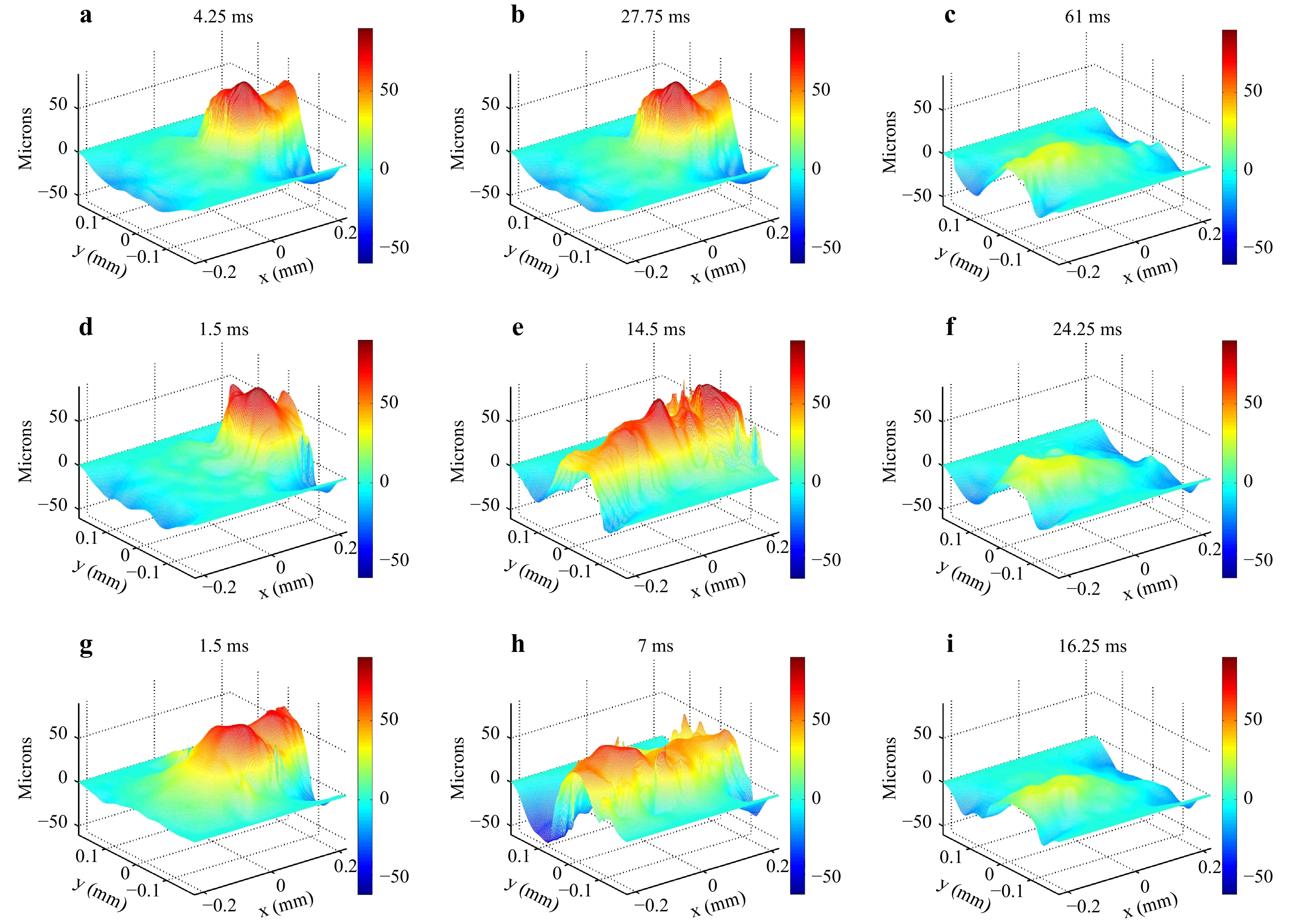

Fig. 6  Topography of dynamic aluminum tracks. a Topography for $ V_0 = \; 100 $ mm·s⁻¹ at 4.25 ms after the beginning of the recording, b at 27.75 ms, c at 61 ms; d topography for $ V_0 = \; 250 $ mm·s⁻¹ at 1.5 ms after the beginning of the recording, e at 14.5 ms, f at 24.25 ms; g topography for $ V_0 = \; 380 $ mm·s⁻¹ at 1.5 ms after the beginning of the recording, h at 7 ms, i at 16.25 ms. Movies: visualization of dynamic aluminum tracks for $ V_0 = \; 100 $ mm·s⁻¹, $ V_0 = \; 250 $ mm·s⁻¹, and $ V_0 = \; 380 $ mm·s⁻¹. Movie 1: visualization of the dynamic tracks for $ V_0 = \; 100 $ mm·s⁻¹; Movie 2: dynamic tracks for $ V_0 = \; 250 $ mm·s⁻¹; Movie 3: dynamic tracks for $ V_0 = \; 380 $ mm·s⁻¹.

Experiments were carried out in open air, and an argon flow from a nozzle was sprayed above the fusion area to reduce the oxidation of the substrate and powder. This means that the melt pool generated during the experiments tended to be unstable. Given that the goal of this study was to realize a proof of concept, it was interesting to evaluate the ability of the holographic system to detect such instabilities. To ensure uniform velocity during fusion, the laser processing was initialized after the start of the motorized stage to avoid any acquisitions during the acceleration phase.

A sheet of 316L plate was used. The exposure time was set to $ \tau = 6.25 $ µs, and the frame rate was 4000 fps. This allowed freezing the dynamic of the melt pool and avoided motion blur in the holograms. The optical magnification was set at $ G_t = 4.29 $, the spatial resolution at the melt pool area was approximately 7.5 µm, obtaining $ B = 0.08 $. Therefore, blur motion was irrelevant. The processing laser had a power of 75 W for a spot diameter between 100 and 200 µm and a velocity of $ V_0 = 100\; $mm·s⁻¹. Under such conditions, a keyhole regime may be observed.

Fig. 7 shows two 3D plots of the topography of the melt pool obtained at two different instants during the laser fire. Fig. 7a displays the melt pool at 87.25 ms, whereas Fig. 7b depicts the melt pool at 88 ms. Fig. 8 shows bottom views corresponding to 3D plots in Fig. 7a, b.

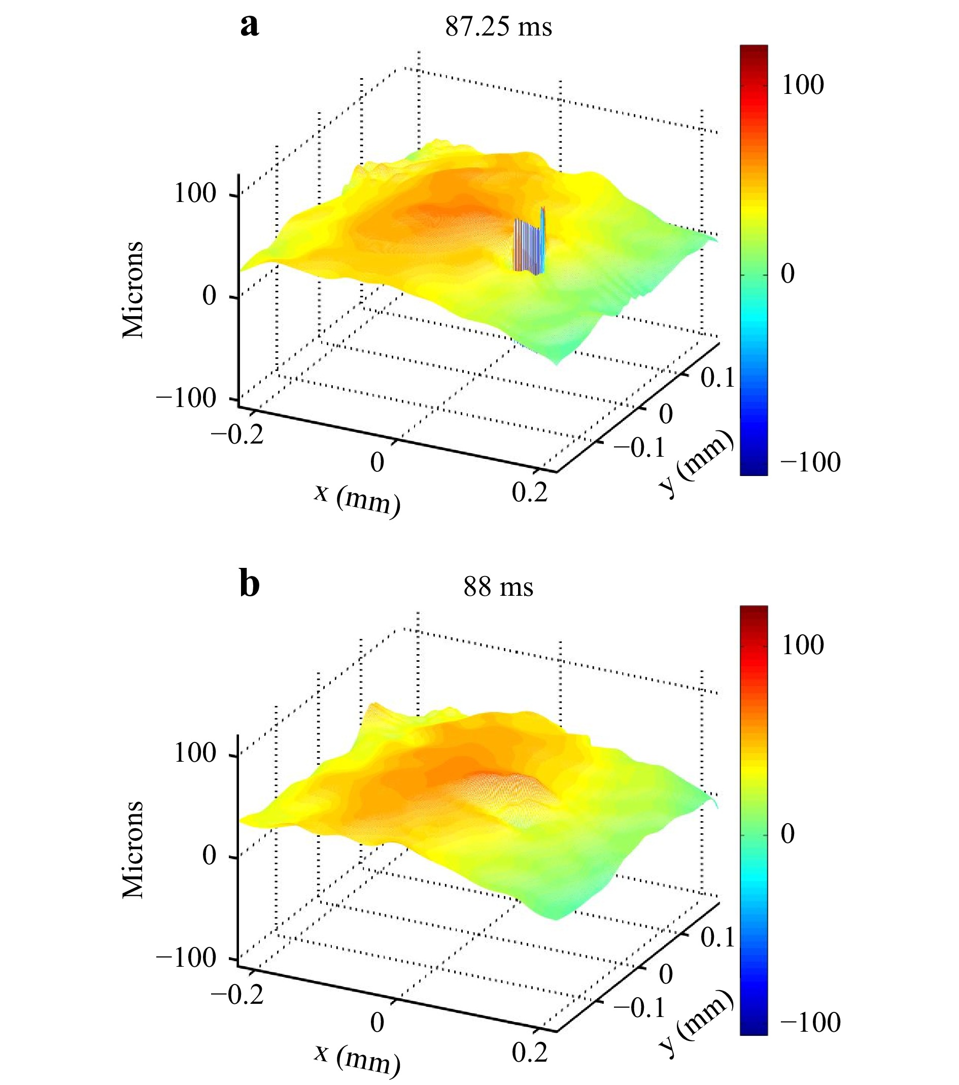
Fig. 7  Monitoring of melt pool on 316L substrate. a 3D plot of melt pool with keyhole at 87.25 ms after the beginning of the recording; b 3D plot of melt pool with keyhole at 88 ms after the beginning of the recording. Laser scanning is along the $ x $ direction.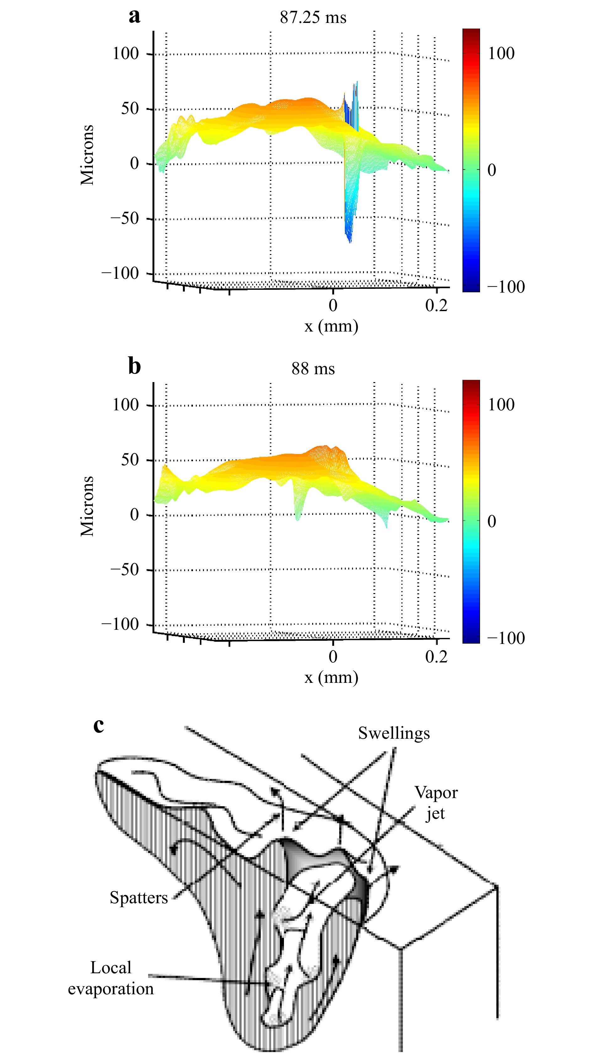

Fig. 8  Keyhole in melt pool on 316L substrate. a Bottom view of melt pool with keyhole at 88 ms after the beginning of the recording; b bottom view of the melt pool with a keyhole at 88 ms after the beginning of the recording; c illustration of the Rosenthal keyhole regime (adapted from Ref. 51). Movie 4: visualization of the keyhole regime.

In this case, a 316L sheet was used with powder 316L. This powder had a thickness of $ \simeq100\; \mu $m and absorbed the laser energy. The melt pool was composed of the fusion of the powder and the fusion of the superficial layer of the substrate. The exposure time was set to $ \tau = 25 $ µs, and the frame rate was 4000 fps. The increase in the exposure time was due to the non-cooperative surface of the 316L powder, which weakly reflects photons. It follows that the hottest area where the keyhole might appear could not be observed owing to the dynamics of the melt pool. The processing laser had a power of 150 W for a spot diameter between 100 and 200 µm and a velocity of $ V_0 = 100\; $ mm·s⁻¹. The optical magnification was set to $ G_t = 4.29 $. Thus, the observed area was approximately 400 × 400 µm². These experimental parameters led to $ B = 0.33 $, which means that the recording was not fully immune to motion blur; this was imposed because of the limited power of the two lasers of the holographic setup.

Fig. 9 shows six pictures of the topography of the melt pool obtained at different instants during the laser melting. The tail and body formation of the melt pool was defined as shown in Fig. 9g.

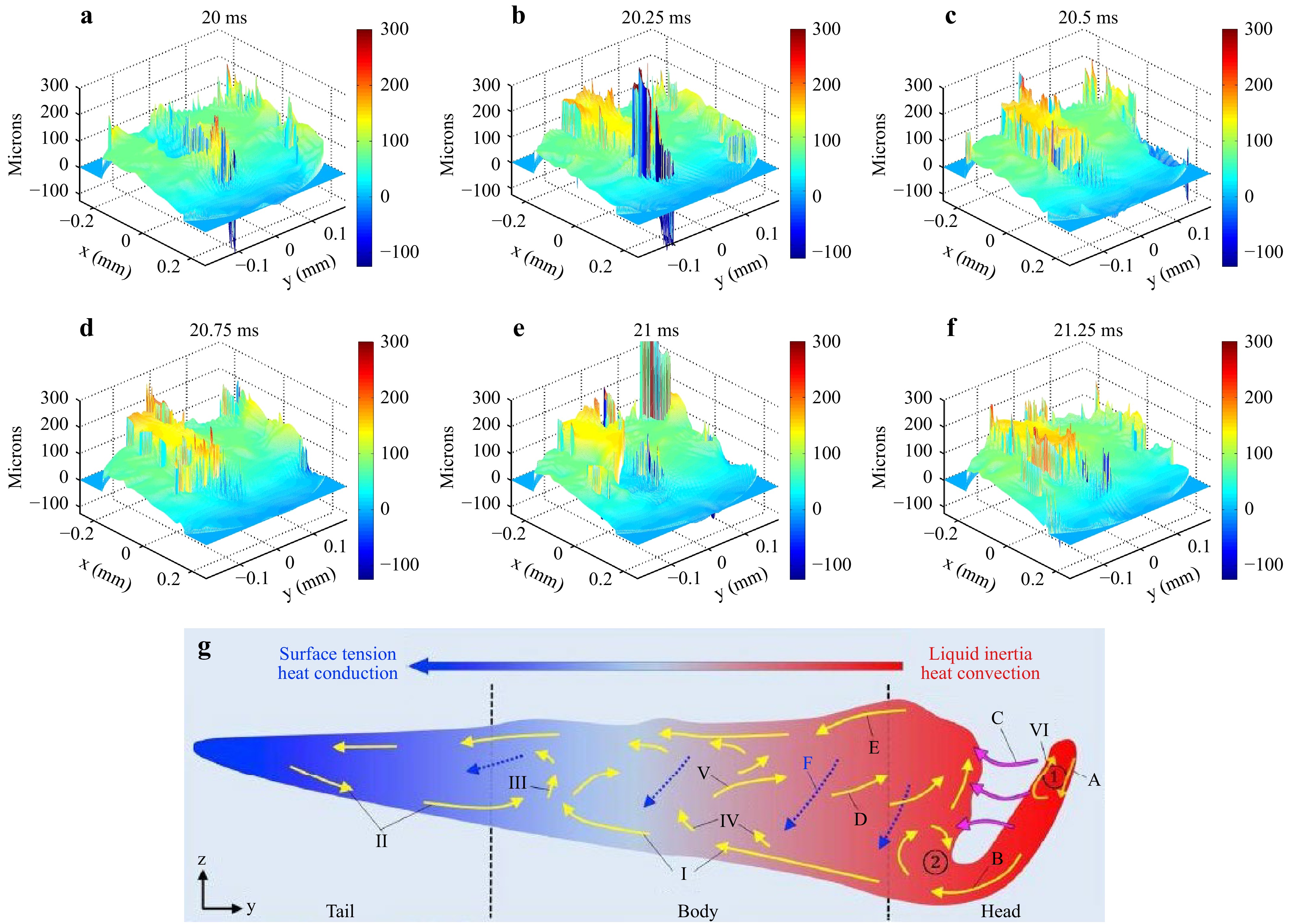
Fig. 9  Topography of melt pool on 316L substrate with 316L powder, a−f several 3D plots at different instants during laser melting, g illustration of melt pool in keyhole mode (adapted from Ref. 41). Movie 5: visualization of the melt pool on 316L substrate with powder

The comparison between the photograph and the tracks in Fig. 5 shows that the topography measured by two-wavelength holography is faithful. The herringbone structure is clearly observable in both the photograph and the topography measurement.

In the following comments on experiments, keep in mind that the processing laser scanned along the $ x $ direction from left to right.

The topographies obtained for the dynamic tracks are shown in Fig. 6, and the respective supplementary movies demonstrate that the holographic setup can yield measurements when the track is scanned at a moderate velocity. Indeed, when the velocity is higher than 100 mm·s⁻¹, motion blur contributes to the degradation of the quality of the measurements. This could be avoided by using more laser power to reduce the exposure time and increase the velocity up to that of industrial processes ($ \simeq\; 1\; $ m·s⁻¹).

Figs. 7−8 permit to visually appraise the depression zone that indicates that the melt pool included the keyhole regime. This regime represents a crucial defect that cannot be identified from thermal radiation monitoring techniques. This regime may be unstable, as can be seen in Fig. 8b, where, at 88 ms, the keyhole regime has disappeared. These results are in good agreement with the description of the keyhole regime proposed by Ge et al⁵². for similar processing conditions. In Fig. 7a, a large variety of surface tension gradients are shown. A deep depression zone characteristic of the keyhole regime was formed at the bottom of the melt pool. The general shape of the melt pool is in agreement with the Rosenthal model represented in Fig. 8c. In Fig. 7b, the melt pool presents a dome shape close to that of the previous view but then enters a transition mode without depression. During the sequence, the melt pool remained unstable and oscillating between these two states^14,53.

When considering melting of the 316L powder on the 316L substrate, Fig. 9 and the supplementary movie show the fluctuations of the melt pool and the establishment of the hot track. These preliminary results demonstrate that monitoring of the melt pool during melting is possible with digital holography, although the results in Fig. 9 are possibly influenced by the motion blur ($ B = 0.33 $) owing to the increase in the exposure time to 25 µs.

This paper proposes two-wavelength digital holography as a proof of concept for real-time in-situ full-field monitoring of melt pools in metal additive manufacturing processes. The holographic system was coupled to a simplified LBM machine, and a high-speed camera was employed to record spatially multiplexed two-color holograms at both temporal and spatial scales of the laser melting process. The surface topography at the melt-pool plane depends on the synthetic wavelength generated by the two wavelengths. The effect of motion blur on the dynamic measurements is discussed. Experimental results are provided: double aluminum tracks on an aluminum substrate, monitoring of dynamic tracks at several velocities, visualization of the keyhole regime on 316L substrate, and visualization of the dynamic melt pool with 316L powder on 316L substrate. To the best of our knowledge, these are the first results of in situ full-field melt pool and track topography in LBM. Although the proof of concept was successful, several improvements are required to increase the performance of the setup. The main point is related to the increase in the laser power of the two probe beams. Indeed, more power for the holographic measurement will achieve better efficiency because more photons could be collected from the melt-pool area, especially if the target has a non-cooperative surface (e.g., the 316L powder used in this study). This is also in good agreement with the possibility of reducing the exposure time of the sensor to a few hundred nanoseconds in order to be fully immune to motion blur. This would be of great interest to reduce the motion blur from the displacement as well as that from the intrinsic dynamics of the melt pool along the $ z $ axis. From a computational point of view, processing of digital holograms, including phase extraction, noise reduction, and unwrapping, requires optimization through the use of a GPU to reduce the calculation time and to rapidly deliver useful data after recording. This study demonstrates that digital holography provides a new opportunity to optimize in situ additive manufacturing processes and develop reliable numerical models to understand the dynamics of the melting process.

This study was carried out in the framework of a research program at ONERA, the French Aerospace Lab, and a PhD program co-funded by Direction Générale de l’Armement (DGA). It was also carried out in collaboration with the Laboratory Procédés et Ingénierie en Mécanique et Matériaux (CNRS 8006) from Arts et Metiers Institute of Technology (Paris, France). The authors are grateful to Frédéric Coste, Pierre Lapouge, and Patrice Peyre for helpful discussions. The authors would like to thank Joseph Montri for his help during the experiments. Special acknowledgement to Alain Appriou for his valuable support.