Phase microscopy and surface profilometry by digital holography

Surface profilometry is an essential technology in many fields of industry such as micro-electronics fabrication and precision machining, as well as in biomedicine. Traditional mechanical stylus-based scanners are largely replaced by non-contact optical methods, such as using patterned illumination, multi-view triangulation, and white light interference¹. Digital holography is a new candidate for high speed, high precision profilometry, due to its ability to reconstruct both the amplitude and the phase of the full optical field. The phase profile of the hologram is directly proportional to the optical path length, such as from transmission through the thickness of a material or reflection off a surface². This is the basis of many applications of quantitative phase microscopy by digital holography, such as cellular microscopy^{3, 4}, micro-device diagnostics⁵, and microfluidics⁶, to name a few.

The complex, i.e. amplitude and phase, field profile is extracted from the interference intensity patterns by off-axis or phase-shifting digital holography⁷. The optical phase is proportional to the optical path length, but only up to modulo $ 2\pi $, and therefore the measured optical path length is ambiguous modulo one wavelength. The so-called phase unwrapping is a common problem in any phase imaging systems, and many numerical phase unwrapping algorithms have been developed⁸, which are typically based on subjective decisions regarding locations of phase discontinuity, and tend to be non-deterministic, unpredictable, and computationally heavy. A technique called optical phase unwrapping has been introduced⁹⁻¹¹, based on combination of several holograms acquired with different wavelengths, that generates phase profiles with effective wavelength¹² much larger than the original wavelengths. The method is completely deterministic and computationally straightforward, and works well even when phase topology is complicated.

The effective, or synthetic, wavelength can be made very large by choosing two closely spaced wavelengths, but this entails proportionate amplification of any noise in the resulting optical path profile. It then becomes necessary to acquire and combine additional holograms with a third, fourth, or more wavelengths, and the noise is reduced in an iterative process described below. The larger the height range to be measured or the more severe the noise level, the more number of wavelengths and holograms is required. The multi-wavelength digital holography (MWDH) has been proposed and demonstrated using a dye laser tuned at three different wavelengths¹³, a tunable diode laser at seven different wavelengths¹⁴, or three discrete lasers¹⁵, for example.

But the use of more than two or three wavelengths becomes increasingly difficult because of the complexity and cost of the optical system, as well as possible chromatic aberration over large range of wavelengths¹⁶. On the other hand, it has been noted early on that a shift in object illumination angle can also have a similar effect as a wavelength shift, because of the variation in the optical path length through a given height or thickness of the object¹⁷. Instead of a set of multiple lasers or scanning of a tunable laser, the angular direction of illumination is scanned to multiple positions to achieve essentially the same effect as with multiple wavelengths.

This article reports a series of studies on optical phase unwrapping based on multi-wavelength digital holography (MWDH) or multi-angle digital holography(MADH) for potential applications in surface profiling with millimeter-scale axial range and micrometer-range axial resolution. In MWDH studies, up to four wavelengths, from as many discrete lasers, are used to generate surface profiles with several mm height range and several $ \mu {\rm{m}} $ height resolution. In MADH studies, it is possible to apply as many as eight different effective wavelengths with a much simpler and flexible optical system. The experimental results are summarized in Section 2. Discussions in Section 3 include comparison of the MWDH and MADH systems. These systems are also described in comparison with a few other related but distinct systems that utilize multi-wavelength or multi-angle acquisition of holograms. Section 4 describes the theoretical background and experimental system and processes.

For illustration of basic processes of four-wavelength MWDH in Fig. 1, the object consists of a pair of glass plates with resolution target patterns with the step size between them measured to be 1.54 mm. As detailed in Materials and Methods, a set of four holograms are acquired by phase-shifting digital holography using four lasers with wavelengths $ {\lambda _1} = 0.639\;616\;\mu {\rm{m}} $, $ {\lambda _2} = $$ 0.639\;595 \; \mu {\rm{m}} $, $ {\lambda _3} = 0.639\;539 \; \mu {\rm{m}} $, and $ {\lambda _4} = 0.638\;929 \; \mu {\rm{m}} $. Fig. 1a, b display the first two phase profiles $ {\Phi _1}\left({x,y} \right) $ and $ {\Phi _2}\left({x,y} \right) $. Because of the minute difference of 0.000 025 $ \mu {\rm{m}} $ between the two wavelengths, any difference between the two phase profiles is not easily discernable. Take the difference between the two phase profiles, modulo $ 2\pi $, and rescale with the synthetic wavelength ${\Lambda _{12}} = {\lambda _1}{\lambda _2}/\left| {{\lambda _1} - {\lambda _2}} \right| $, to obtain the height profile $ {Z_{12}} $. The three-dimensional shape of the object then becomes apparent, shown in Fig. 1c, as well as the step between the two glass plates in Fig. 2a. The set of parameters used in this experiment is tabulated in Table 1.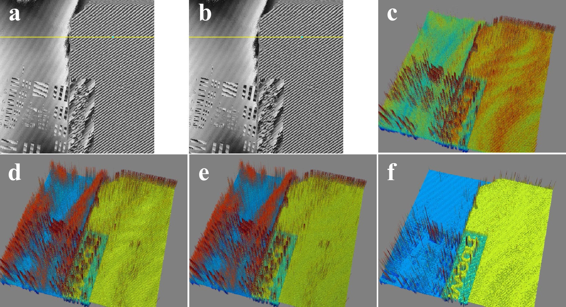

Fig. 1  Basic process of optical phase unwrapping by MWDH using four wavelengths, tabulated in Table 1. The object is a stack of two resolution target surfaces, with field of view $ 24 \times 24\,{\rm{m}}{{\rm{m}}^2}. $ a $ {\Phi _1}\left({x,y} \right) $; b $ {\Phi _2}\left({x,y} \right) $; c $ {Z_{12}}\left({x,y} \right) $; d $ {Z_{12 \cdots 3}}\left({x,y} \right) $; e $ {Z_{12 \cdots 4}}\left({x,y} \right) $; f $ {Z_{{\rm{proc}}}}\left({x,y} \right) $. See Fig. 2 for indication of the z-scale. See text for details.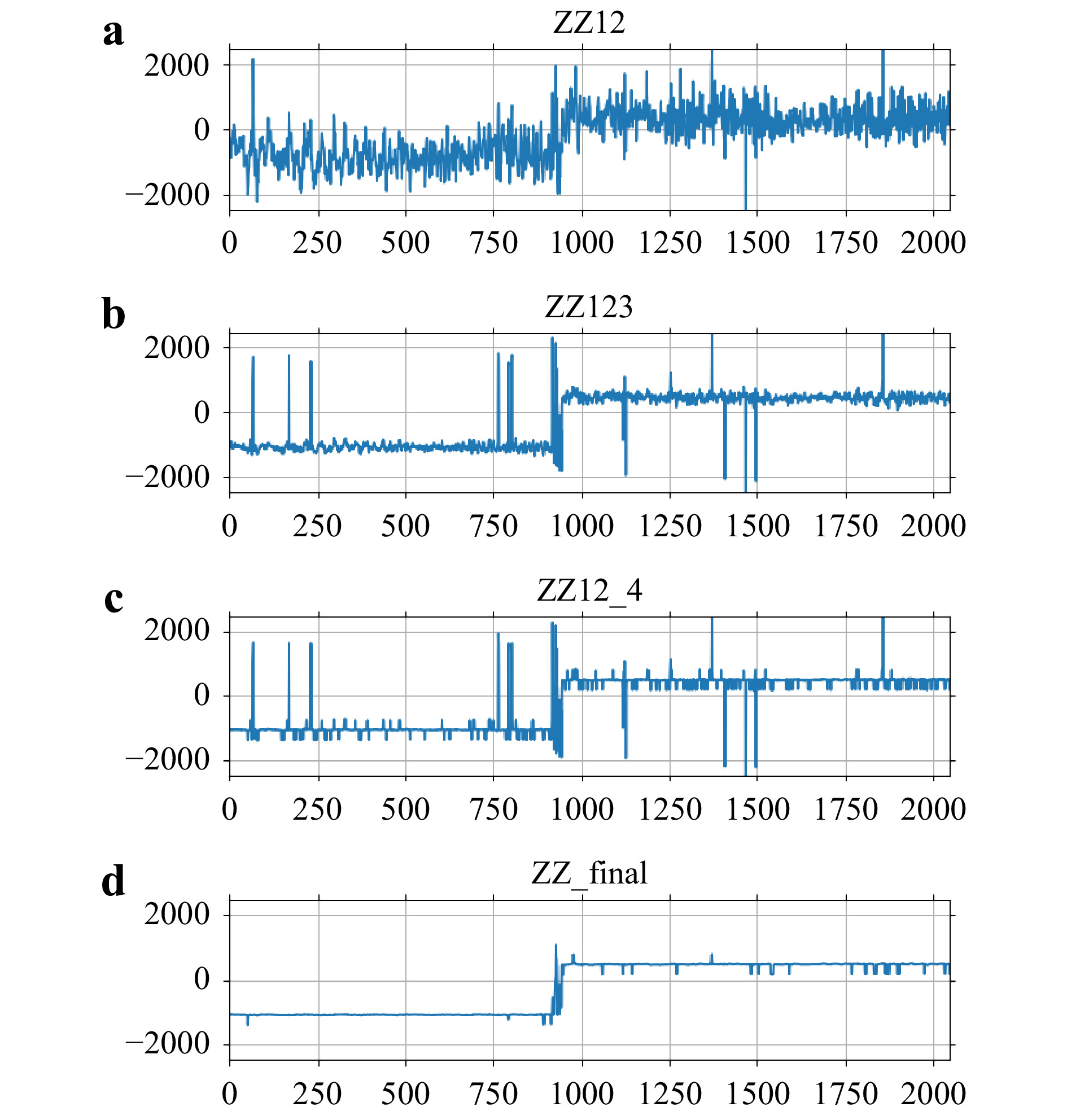

Fig. 2  Graphs of cross-sections of a $ {Z_{12}} $; b $ {Z_{12 \cdots 3}} $; c $ {Z_{12 \cdots 4}} $; d $ {Z_{{\rm{proc}}}} $, through the yellow line indicated in Fig. 1a. The vertical scales, in $ \mu {\rm{m}} $, are multiplied by a factor 0.5 to account for the reflection geometry. The horizontal scale is the pixel index. A $ 3 \times 3 $ median filter is applied to $ {Z_{{\rm{12}} \cdots {\rm{4}}}} $ to obtain $ {Z_{{\rm{proc}}}} $. Measured height noise is tabulated in Table 1. The measured step height is 1.55 mm, comparable to the 1.54 mm nominal glass thickness.

The difference of the two phase profiles corresponds to another phase profile with very large synthetic wavelength $ {\Lambda _{12}} = 19\; 749 \; \mu {\rm{m}} $, amplifying the wavelength by a factor of $ {\Lambda _{12}}/{\lambda _1} \approx 3 \times {10^4} $. The difference phase map has the same level of phase noise, other than a factor of order one, as the initial phase maps, meaning that with the amplification of effective wavelength, the noise in the height profile is also amplified by the same factor. In Fig. 2a, the noise in the height profile is measured to be $ \delta {Z_{12}} = 919.1 \; \mu {\rm{m}} $, and the 3D profile in Fig. 1c shows significant amount of rough and spiky textures on the surfaces. Significant reduction in noise is achieved by iterative stitching of additional difference phase profiles $ {Z_{13}} $ and $ {Z_{14}} $ with shorter synthetic wavelengths $ {\Lambda _{13}} = 5\;302 \;\mu {\rm{m}} $ and $ {\Lambda _{14}} = 595 \; \mu {\rm{m}} $, respectively. The stitching process maintains the overall height range to $ {\Lambda _{12}} $ while reducing the noise to the proportionately lower levels of $ {Z_{13}} $ and $ {Z_{14}} $, whose measured noise in Fig. 2d, e are $ \delta {Z_{13}} = 564.9 \;\mu {\rm{m}} $ and $ \delta {Z_{14}} = 593.2 \;\mu {\rm{m}} $, respectively. The last stitching operation with $ {Z_{14}} $ has no apparent improvement in the measured noise because the reduction in synthetic wavelength is too rapid. The necessary condition is given in the Materials and Methods section, but with the given set of laser wavelengths, there is no flexibility in the choice of wavelengths. On the other hand, as we will see, the generation of effective wavelength can be made very flexible by varying the object illumination angle instead. A common and effective method of reducing spiky noise is using median filters. A mild median filter with $ 3 \times 3 $ window is applied to the last profile $ {Z_{12 \cdots 4}} $ of the iterative series to obtain the final processed profile $ {Z_{{\rm{proc}}}} $ in Fig. 1f and Fig. 2d, where the corresponding noise is reduced to $ \delta {Z_{{\rm{proc}}}} = 101.7 \;\mu {\rm{m}} $. The measured step height in $ {Z_{{\rm{proc}}}} $ is 1.55 mm, consistent with the nominal thickness of the glass plate.

In Fig. 3, 4, a similar set of parameters is used to image the surface of a US quarter dollar coin, placed on a mirror-like surface. The synthetic wavelengths used were $ {\Lambda _{12}} = 28\; 213 \;\mu {\rm{m}} $, $ {\Lambda _{13}} = 5\; 302\;\mu {\rm{m}} $, $ {\Lambda _{14}} = 595 \;\mu {\rm{m}} $. The single-wavelength phase profiles in Fig. 3a, b have no discernable features, because of the random granular structure of the metallic surface. Yet the surface profile $ {Z_{12}} $ from the difference profile does reveal the overall features of the surface pattern. The iterative processing with ‘stitching’ is applied as above, and in order to improve the image quality, a $ 3\; \times \;3 $ median filter was applied to each step of $ {Z_{12}} $, $ {Z_{123}} $, and $ {Z_{12 \cdots 4}} $. The noise level, measured over a small smooth area of the coin surface, is reduced from $ \delta {Z_{12}} = 385.0 \; \mu {\rm{m}} $ to $ \delta {Z_{14}} = 3.8 \; \mu {\rm{m}} $. It is seen that final processed images with just a few micrometer noise is achieved with relatively mild application of median filters.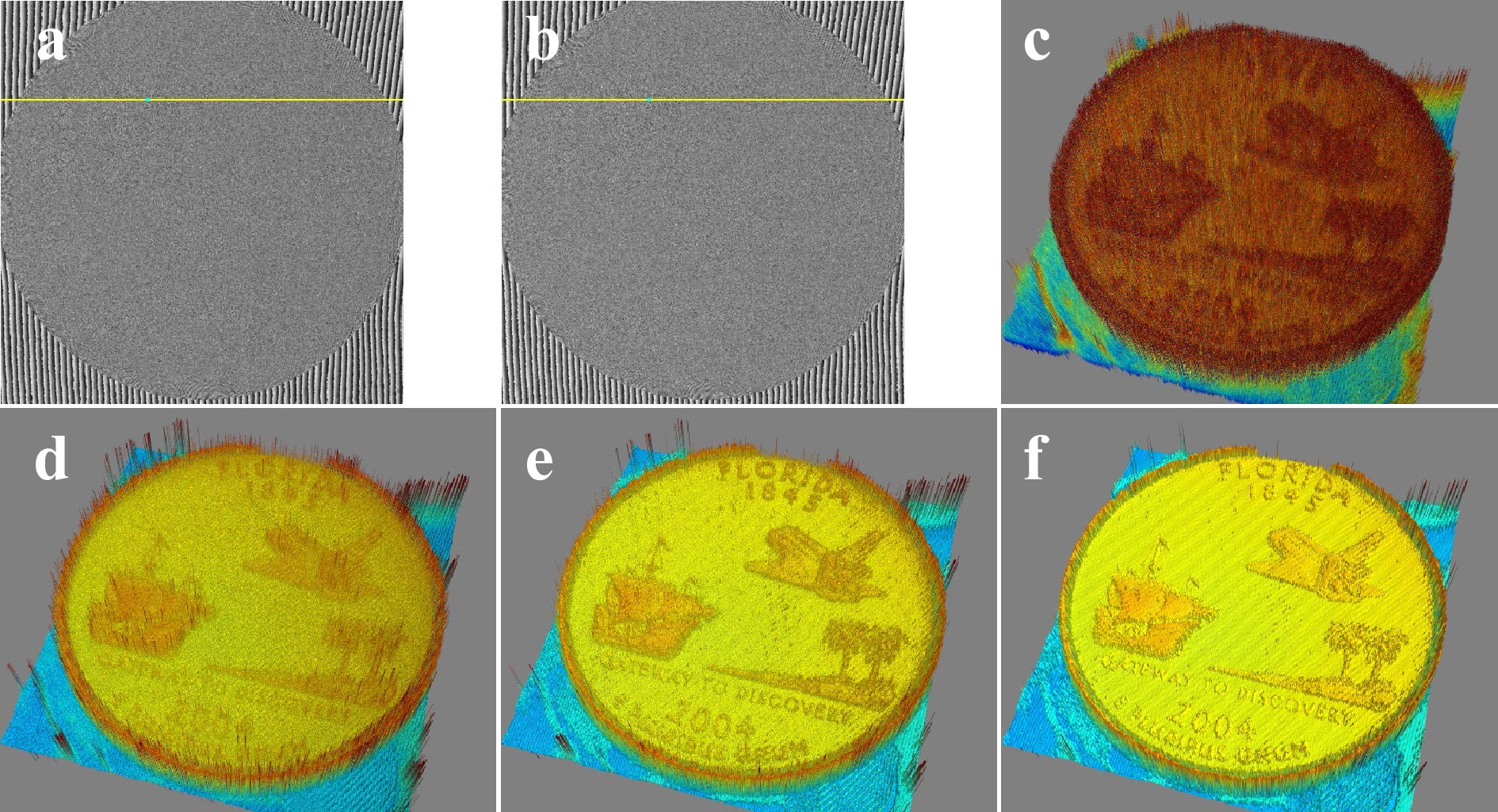

Fig. 3  Example of optical phase unwrapping by MWDH. The object is a US quarter dollar coin, with field of view $ 24 \times 24\;{\rm{m}}{{\rm{m}}^2} $. A set of four wavelengths are used, such that $ {\Lambda _{12}} = 28\; 213 \; \mu {\rm{m}} $, $ {\Lambda _{13}} = 4 \;328 \; \mu {\rm{m}} $, and $ {\Lambda _{14}} = 485 \; \mu {\rm{m}} $. a $ {\Phi _1}\left({x,y} \right) $; b $ {\Phi _2}\left({x,y} \right) $; c $ {Z_{12}}\left({x,y} \right) $; d $ {Z_{12 \cdots 3}}\left({x,y} \right) $; e $ {Z_{12 \cdots 4}}\left({x,y} \right) $; f $ {Z_{{\rm{proc}}}}\left({x,y} \right) $. See Fig. 4 for indication of the z-scale.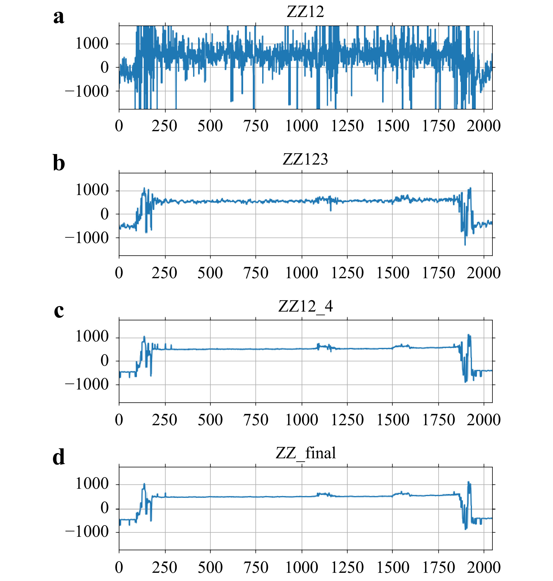

Fig. 4  Graphs of cross-sections of a $ {Z_{12}} $; b $ {Z_{12 \cdots 3}} $; c $ {Z_{12 \cdots 4}} $; d $ {Z_{{\rm{proc}}}} $, through the yellow line indicated in Fig. 3a. The vertical scales, in $ \mu {\rm{m}} $, are multiplied by a factor 0.5 to account for the reflection geometry. The horizontal scale is the pixel index. A $ 3 \times 3 $ median filter is applied to each of $ {Z_{12}} \sim{Z_{12 \cdots 4}} $ and to $ {Z_{{\rm{proc}}}} $. Measured height noise varies as $ \delta {Z_{12}} = 385.0 \; \mu {\rm{m}} $, $ \delta {Z_{12 \cdots 3}} = 22.6 \; \mu {\rm{m}} $, $ \delta {Z_{12 \cdots 4}} = 3.8 \; \mu {\rm{m}} $, and $ \delta {Z_{{\rm{proc}}}} = 3.2 \; \mu {\rm{m}} $.

The process of MADH is illustrated with an example in Fig. 5, 6, where the object consists of a set of three mirror-like surfaces with nominal step heights 1.54 mm and 0.94 mm between them. A set of eight holograms are acquired, using a single HeNe laser of $ {\lambda _0} = 0.632\;8 \; \mu {\rm{m}} $, at illumination angles $ {\theta _n} = {\theta _0} + {\Delta _n} $, tabulated in Table 2. In this experiment, an alternate version of the optical apparatus was used, where the reference beam is stationary and only the object illumination is scanned. The starting position $ {\theta _0} = {18^ \circ } $ corresponds to the case of the object beam coinciding with the reference beam direction, while $ {\Delta _n} $ are precisely controlled by the rotation stage with $ {0.000\;25^ \circ } $ resolution. The first two phase profiles $ {\Phi _1} $ and $ {\Phi _2} $ are displayed in Fig. 5a, b. The patterns indicate slight relative tilt between the three surfaces. The angular step $ {\theta _2} - {\theta _1} = {0.0014^ \circ } $ between the first two holograms determines the synthetic wavelength $ {\Lambda _{12}} = 7\; 545 \;\mu {\rm{m}} $, with the effective wavelengths $ {\lambda _n} = {\lambda _0}\cos {\theta _n} = 0.601\; 829 \;\mu {\rm{m}} $ and $0.601\; 781\; \mu {\rm{m}} $, for $ n = 1$ and 2, repectively. Additional angular steps $ {\theta _n} - {\theta _1} $, which increase by a factor of two in each step in this example, lead to synthetic wavelengths $ {\Lambda _{1n}} $ that decrease by a factor of $ \alpha \approx 0.50 $, each step for $ n > 2 $. The ‘stitching’ process is iterably applied with the series of profiles $ {Z_{13}}, \cdots,{Z_{18}} $. The noise levels $ {\delta _{1n}} $ of the ‘stitched’ maps $ {Z_{12 \cdots n}} $, in Fig. 5, 6 are measured as the standard deviation of a small area near the center of the frame. They progressively decrease by a factor close to α each step, while maintaining the overall height range $ {\Lambda _{12}} $. The surface profiles rendered as 3D plots in Figs. 5c−f show obvious enhancement of image quality between $ {Z_{12}} $ and $ {Z_{12 \cdots 8}} $, as the noise decreases from $ \delta {Z_{12}} = 127.4 \; \mu {\rm{m}} $ to $ \delta {Z_{18}} = 3.5 \;\mu {\rm{m}} $, with $ \delta {Z_{18}}/\delta {Z_{12}} = 0.027\;5 = {\alpha ^{5.18}}$, consistent with the expected factor of $ {\alpha ^{n - 2}} $. In this case, the noise reduction is quite complete throughout the surface except at the steps because of the beveled edges reflecting insufficient light towards the camera. With application of a mild $ 3 \times 3 $ median filter on the last stitched profile $ {Z_{12 \cdots 8}} $, a final noise level of $ \delta {Z_{{\rm{proc}}}} = 2.0 \; \mu {\rm{m}} $ is achieved over a height range of $ {\Lambda _{12}} = 3\; 758 \; \mu {\rm{m}} $.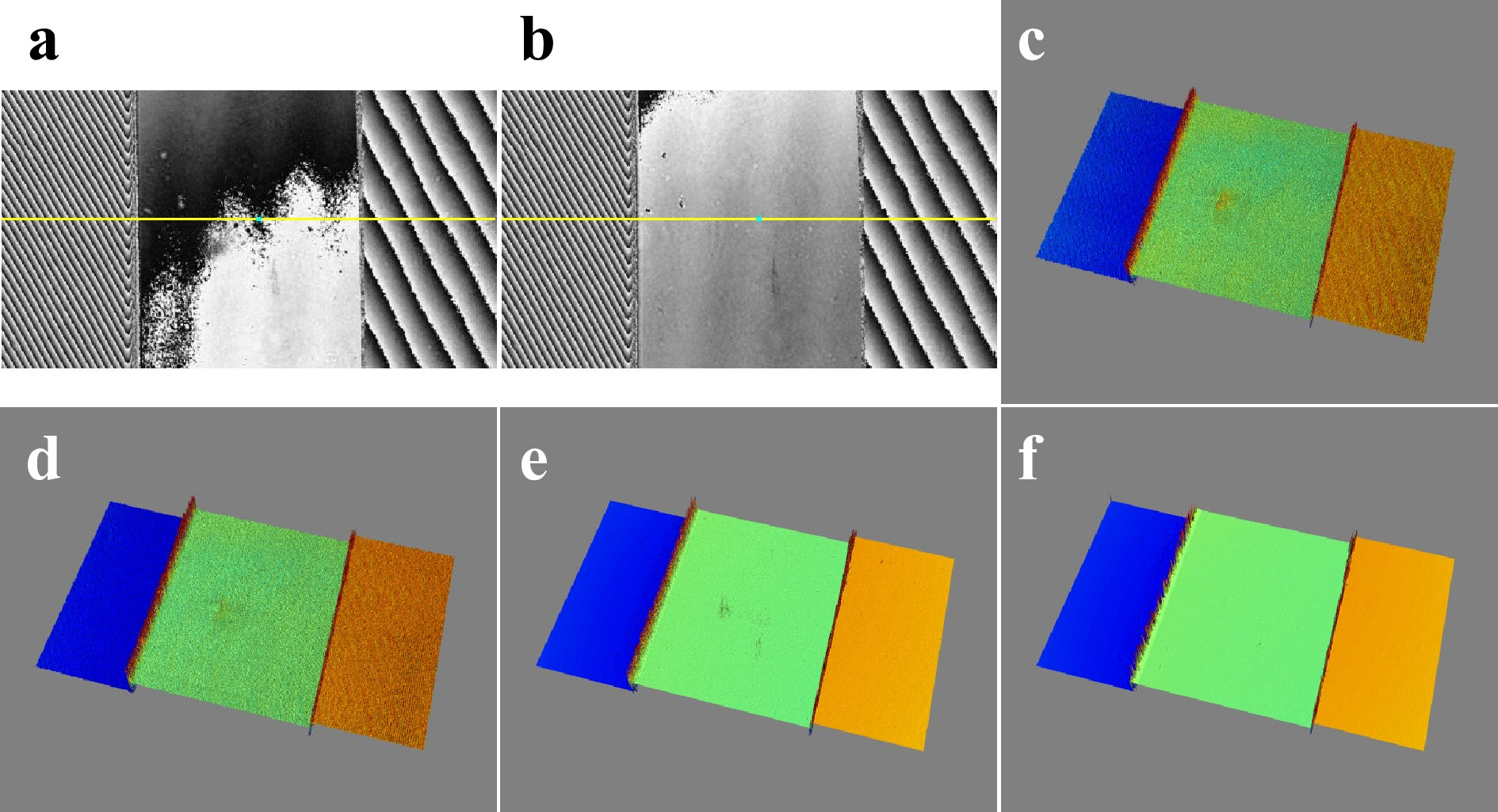

Fig. 5  Basic process of optical phase unwrapping by MADH using eight illumination angles for eight effective wavelengths, tabulated in Table 2. The object is a stack of three mirror-like surfaces, with field of view $ 9.87 \times 5.55\,{\rm{m}}{{\rm{m}}^2} $. a $ {\Phi _1}\left({x,y} \right) $; b $ {\Phi _2}\left({x,y} \right) $; c $ {Z_{12}}\left({x,y} \right) $; d $ {Z_{12 \cdots 3}}\left({x,y} \right) $; e $ {Z_{12 \cdots 8}}\left({x,y} \right) $; f $ {Z_{{\rm{proc}}}}\left({x,y} \right) $. Plots for $ {Z_{12 \cdots 4}} $ through $ {Z_{12 \cdots 7}} $ are not displayed. See text for details. See Fig. 6 for indication of the z-scale.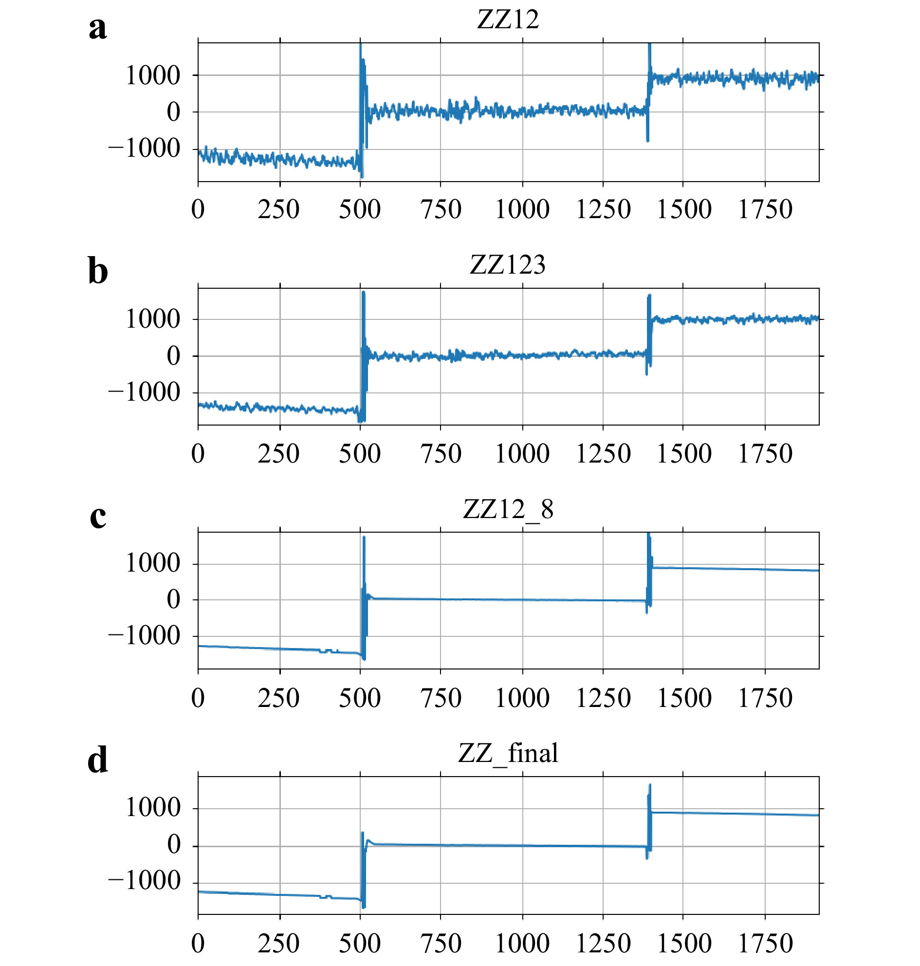

Fig. 6  Graphs of cross-sections of a $ {Z_{12}} $; b $ {Z_{12 \cdots 3}} $; c $ {Z_{12 \cdots 8}} $; d $ {Z_{{\rm{proc}}}} $, through the yellow line indicated in Fig. 5a. The vertical scales, in $ \mu {\rm{m}} $, are multiplied by a factor 0.5 to account for the reflection geometry. The horizontal scale is the pixel index. Graphs for $ {Z_{12 \cdots 4}} $ through $ {Z_{12 \cdots 7}} $ are omitted. A $ 3 \times 3 $ median filter is applied to $ {Z_{{\rm{12}} \cdots {\rm{8}}}} $ to obtain $ {Z_{{\rm{proc}}}} $. Measured height noise is tabulated in Table 2. The measured step heights are 1.56 mm and 0.97 mm, comparable to the nominal glass thicknesses of 1.54 mm and 0.95 mm.

Fig. 7, 8 is an example surface profile of a coin (U.S. penny) placed on another (U.S. quarter). Here a set of eight holograms are acquired using the stepping factor $ \alpha = 0.50 $ for the synthetic wavelengths ranging from $ {\Lambda _{12}} = 2 \;911.5 \;\mu {\rm{m}} $ to $ {\Lambda _{18}} = 44.1 \;\mu {\rm{m}} $. Because of the microscopically diffuse surface of the coin, as well as the slopes on the boundaries of the letters and relief features, there is significant noise in the raw profile $ {Z_{12}} $, shown in Fig. 7c, 8a. The relatively small numerical aperture of the system, approx. 0.1, is not able to collect enough light from these sloped boundary surfaces for accurate phase information. The same stitching procedure as above is applied using the series $ {Z_{13}}, \cdots,{Z_{18}} $, but after each step a $ 3\; \times\; 3 $ median filter is applied. This produced reasonably clean surface profile of the coin without noticeable degradation or loss of lateral resolution. The measured noise reduced from $ \delta {Z_{12}} = 147.3 \; \mu {\rm{m}} $ to $ \delta {Z_{18}} = 10.4 \; \mu {\rm{m}} $.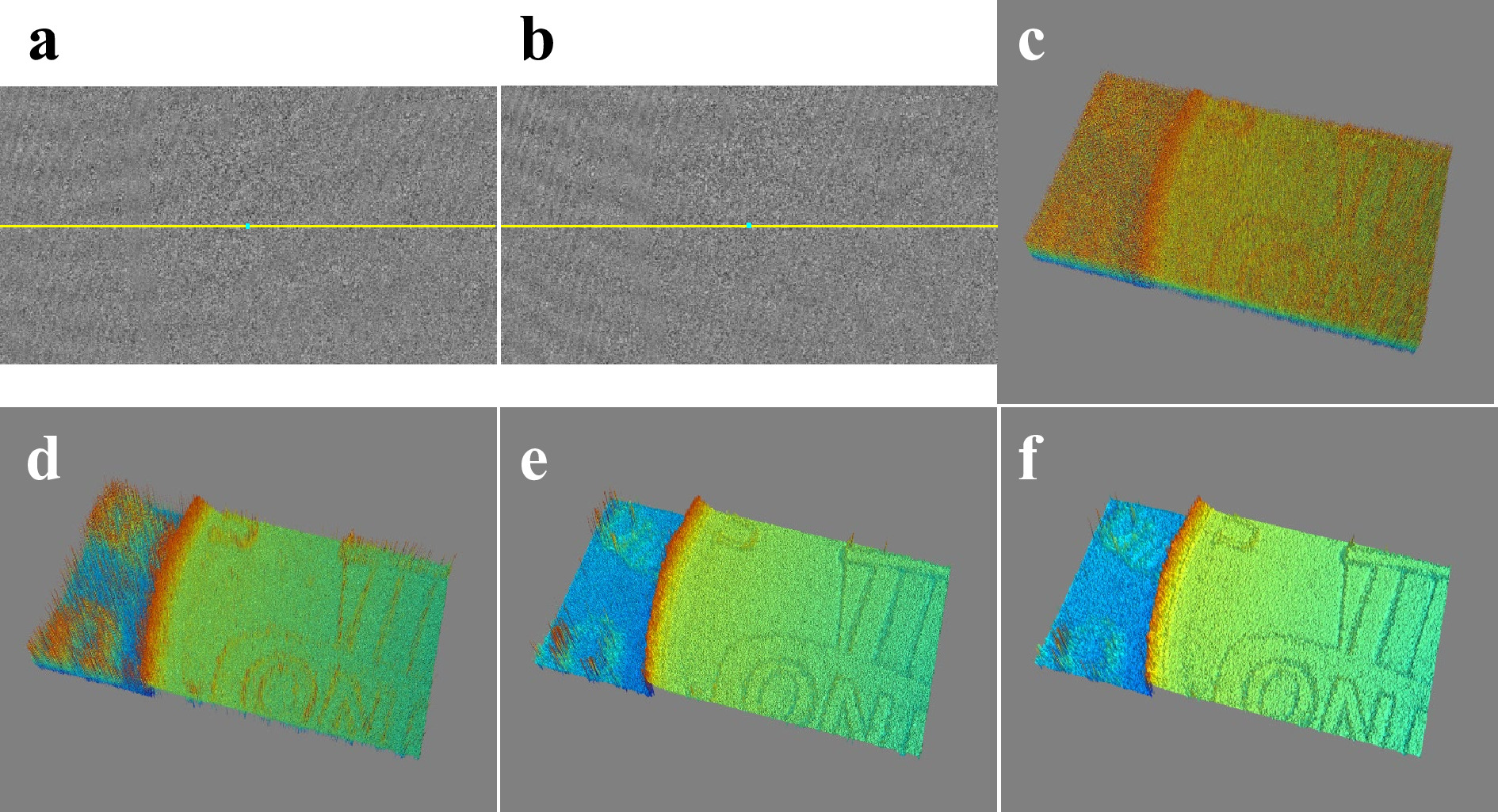

Fig. 7  Example of optical phase unwrapping by MADH. The object is a coin, US penny, placed on top of another, a US quarter, with field of view $ 9.87 \times 5.55\,{\rm{m}}{{\rm{m}}^2} $. A set of eight wavelengths are used, such that $ {\Lambda _{1n}} = [2\; 911.5, 1\; 455.5, 727.5, 363.5, 180.9, 89.7, 44.1] \;\mu {\rm{m}} $ for $ n = 2,\,3,\, \cdots,\,8 $. a $ {\Phi _1}\left({x,y} \right) $; b $ {\Phi _2}\left({x,y} \right) $; c $ {Z_{12}}\left({x,y} \right) $; d $ {Z_{12 \cdots 3}}\left({x,y} \right) $; e $ {Z_{12 \cdots 8}}\left({x,y} \right) $; f $ {Z_{{\rm{proc}}}}\left({x,y} \right) $. See Fig. 8 for indication of the z-scale.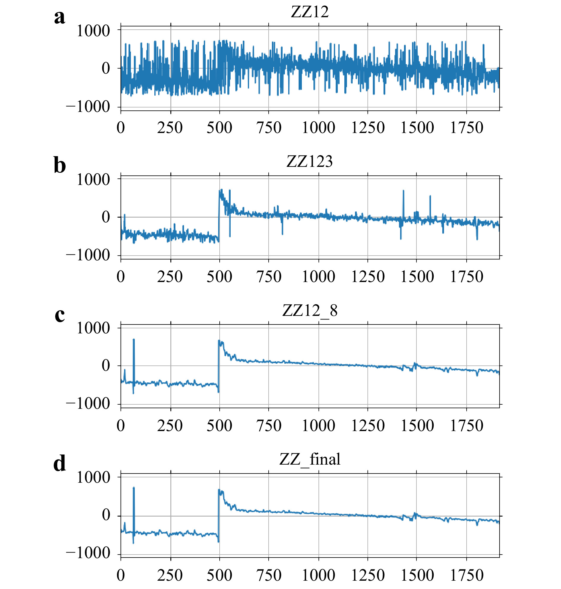

Fig. 8  Graphs of cross-sections of a $ {Z_{12}} $; b $ {Z_{12 \cdots 3}} $; c $ {Z_{12 \cdots 8}} $; d $ {Z_{{\rm{proc}}}} $, through the yellow line indicated in Fig. 7a. The vertical scales, in $ \mu {\rm{m}} $, are multiplied by a factor 0.5 to account for the reflection geometry. The horizontal scale is the pixel index. A $ 3 \times 3 $ median filter is applied to each of $ {Z_{12}} \sim{Z_{12 \cdots 8}} $ and to $ {Z_{{\rm{proc}}}} $. Measured height noise varies as $ \delta {Z_{12 \cdots n}} = [147.3, 29.5, 27.2, 23.2, 15.5, 13.9, 10.4] \; \mu {\rm{m}} $ for $ n = 2,\,3,\, \cdots,\,8 $, and $ \delta {Z_{{\rm{proc}}}} = 9.0 \; \mu {\rm{m}} $.

As described in Section 4, there is a limit on how fast the iterative noise reduction can progress, i.e. how small the stepping factor α can be. For larger amount of initial noise, the stepping factor cannot be chosen too small, for otherwise the iterative noise reduction can become incomplete. To illustrate, in Fig. 9, the same coin surface data as in Fig. 8 is used, but instead of stitching all of the profiles $ {Z_{13}}, \cdots,{Z_{18}} $ on to $ {Z_{12}} $, only the partial set of $ {Z_{12}} $, $ {Z_{15}} $, and $ {Z_{18}} $ is used for stitching. Here, $ Z\left({12} \right) $, $ Z\left({12 + 15} \right) $, and $ Z\left({12 + 15 + 18} \right) $, denote $ {Z_{12}} $, it stitched with $ {Z_{15}} $, and the last stitched with $ {Z_{18}} $, respectively. This in effect reduces the stepping factor to $ \alpha = 0.125$. Otherwise the same set of processing procedure is applied as with Fig. 8, including the $ 3 \times 3 $ median filter at each stitching step. The stepping factor is too small and the iteration is too fast, and significant amount of noise escapes the reduction procedure, the final noise level being 34 $ \mu {\rm{m}} $ for $ \alpha = 0.125$, compared to 9.0 $ \mu {\rm{m}} $ for $ \alpha = 0.50$.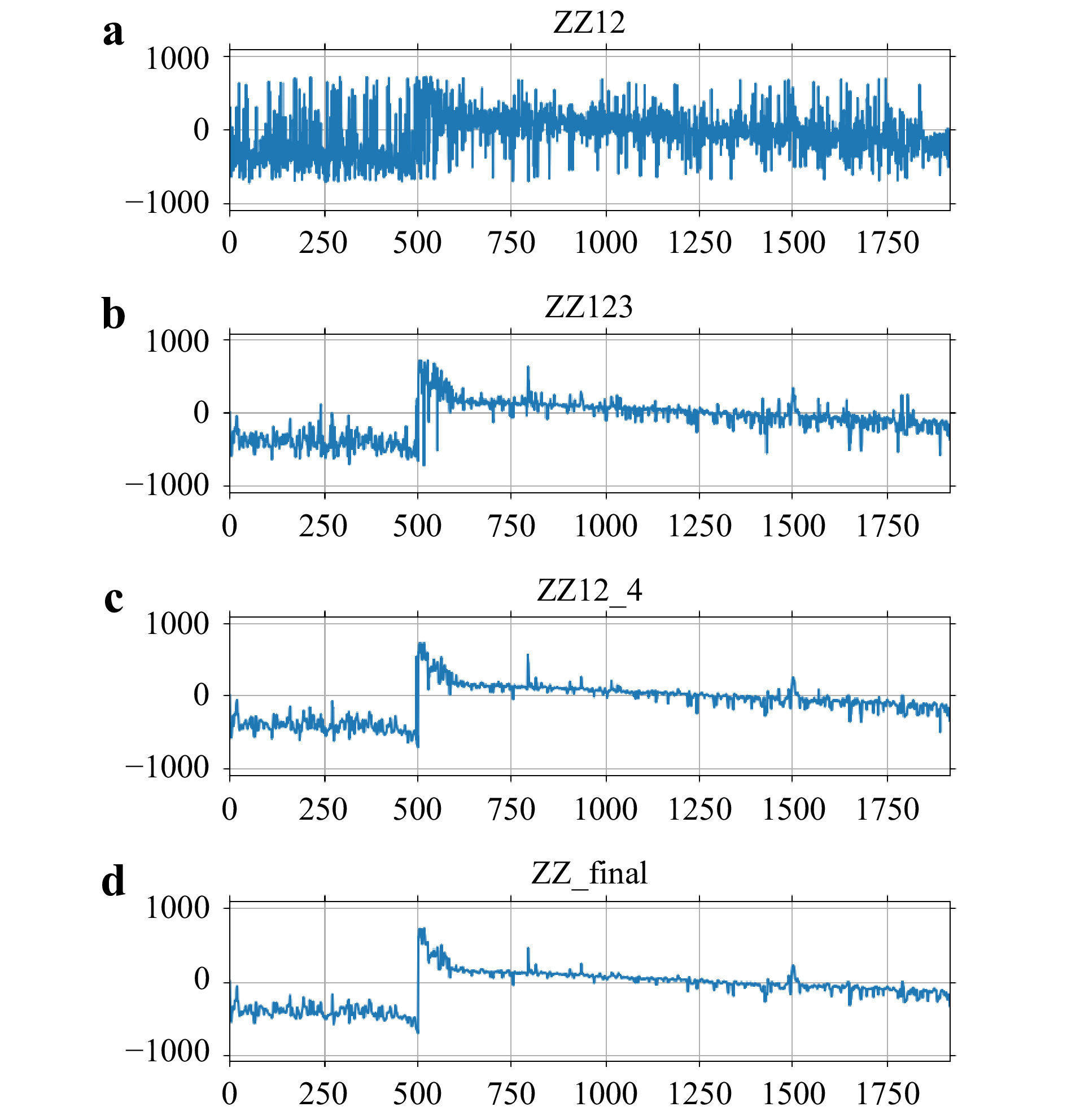

Fig. 9  Effect of iteration being too rapid with $ \alpha = 0.125 $. Graphs of cross-sections of a $ Z\left({12} \right) $; b $ Z\left({12 + 15} \right) $; c $ Z\left({12 + 15 + 18} \right) $; d $ {Z_{{\rm{proc}}}} $. The vertical scales, in $ \mu {\rm{m}} $, are multiplied by a factor 0.5 to account for the reflection geometry. The horizontal scale is the pixel index. A $ 3 \times 3 $ median filter is applied to each profile. Measured height noise varies as $ \delta {Z_{12}} = 147.3 \; \mu {\rm{m}} $, $ \delta {Z_{12 + 15}} = 58.7 \; \mu {\rm{m}} $, $ \delta {Z_{12 + 18}} = 42.2 \; \mu {\rm{m}} $, and $ \delta {Z_{{\rm{proc}}}} = 34.1 \; \mu {\rm{m}} $. See text for details.

A few more examples of surface profiles are given in Fig. 10, by optical phase unwrapping with MWDH or MADH. Imaging parameters of the examples are summarized in Table 3.

Fig. 10  Examples of MWDH and MADH images. Imaging parameters are tabulated in Table 3.

The median filter is quite effective in removing the spiky noise. For some of the examples presented in Section 2, such as coin surfaces, application of simple $ 3\; \times\; 3 $ median filter a few times was sufficient to produce good-quality surface profiles. For more rough textured surfaces such as integrated circuit chips and printed circuit boards, heavier dose of filtering was necessary, such as $ 10 \sim 20\; \times $ repeated applications of $ 3 \;\times\;3 $ median filter. Some loss of surface details is inevitable, but it seems to be justified by the improvement in overall quality of the final image. It is also found useful in some cases to adjust the median filter to larger window size for darker areas of the amplitude image, and vice versa. Such adaptive median filter (AMF) technique was used to obtain the images in Figs. 10a−c, and helped reduce strong noise in corners and metallic electrodes.

Several other denoising methods were attempted from collection of ‘conventional’ image processing tools, such as windowed Fourier transform (WFT), total variation denoising (TVD), non-local means filtering(NLMF), and block-matching and 3D filtering (BM3D)¹⁸, as well as random mask multi-look (RMML) method for holographic speckle processing¹⁹. These somewhat casual studies did not find a magic solution for general applications, but each technique tends to be applicable only to specific cases, pose substantial computational load, and cause significant degradation of details. The behavior of spiky noise in this type of stitched phase maps appear very different from typical noise in photographic images or the speckle noise in holographic intensity images. Further systematic study of the behavior of this new type of noise may be of interest²⁰.

A few points can be made in comparing the methods of MWDH and MADH. First, both methods, when properly set up and carried out, can produce good quality surface profile images. In general, the MADH system has advantage with cost and complexity. The selection of effective wavelengths is very flexible and more controllable. A potential issue is shadowing and obscuration by tall or sharp surface features. The MWDH may be subject to chromatic aberration when the wavelength interval is substantial. The MADH can also be subject to geometric aberration because of the movement of the beam across the optical aperture. If the size of the aberration is more than a few wavelengths, the reconstructed surface profile may include as much distortion. This type of distortion can be compensated for, if necessary, by acquiring a set of blank holograms with a flat mirror in place of the object plane.

There is an alternate approach to unwrapping of quantitative phase images by angular scanning, where small step phase changes are accumulated over many small step anglular shifts²¹. General type and quality of surface profile images may be similar to the method presented here. In principle, in order to achieve the same level of height range and resolution, both methods of this paper and of²¹ start from the same first wavelength $ {\lambda _1} $ and scan to the final synthetic wavelength $ {\lambda _N} $. The method of²¹ takes uniform wavelength steps throughout the scan, while the method of this paper takes progressively larger steps to reach the final wavlength. Direct experimental comparison has not been attempted, but because of the significantly larger number of holographic frames, the acquisition may take longer time and therefore susceptible to instability.

One may also note other related but distinct holographic methods of surface profiling. For example, many holograms are acquired using a range of wavelengths. The stack of holograms is then Fourier transformed along the inverse-of-wavelength axis, which represents the 3D surface topography²². Similar result can be obtained by replacing the wavelength scanning with angular scanning²³⁻²⁵. These processes in effect synthesize temporal incoherence from diversity of frequencies, i.e. inverse of wavelength, either by wavelength scanning or angular scanning. The axial resolution is limited by the synthesized coherence length and in principle significantly lower than the sub-wavelength axial resolution of phase profile-based methods presented here.

These demonstration experiments validate the basic concept of optical phase unwrapping and iterative noise reduction by multi-wavelength and multi-angle digital holography. With the quantitative phase method presented here, high resolution surface profiles can be obtained with large unambiguous range, while maintaining close to single-wavelength axial resolution. Further work is in progress, in particular with respect to the novel behavior of phase noise in this type of quantitative phase imaging system, as well as development of profilometry applications in device fabrication and biomedical imaging.

The basic process of multi-wavelength optical phase unwrapping is illustrated with simulations in Fig. 11. Suppose the object is an inclined plane of height $ {a_h} = 15 \; \mu {\rm{m}} $, depicted with the function $ h\left(x \right) $ in Fig. 11a, and a set of holograms are acquired using a series of wavelengths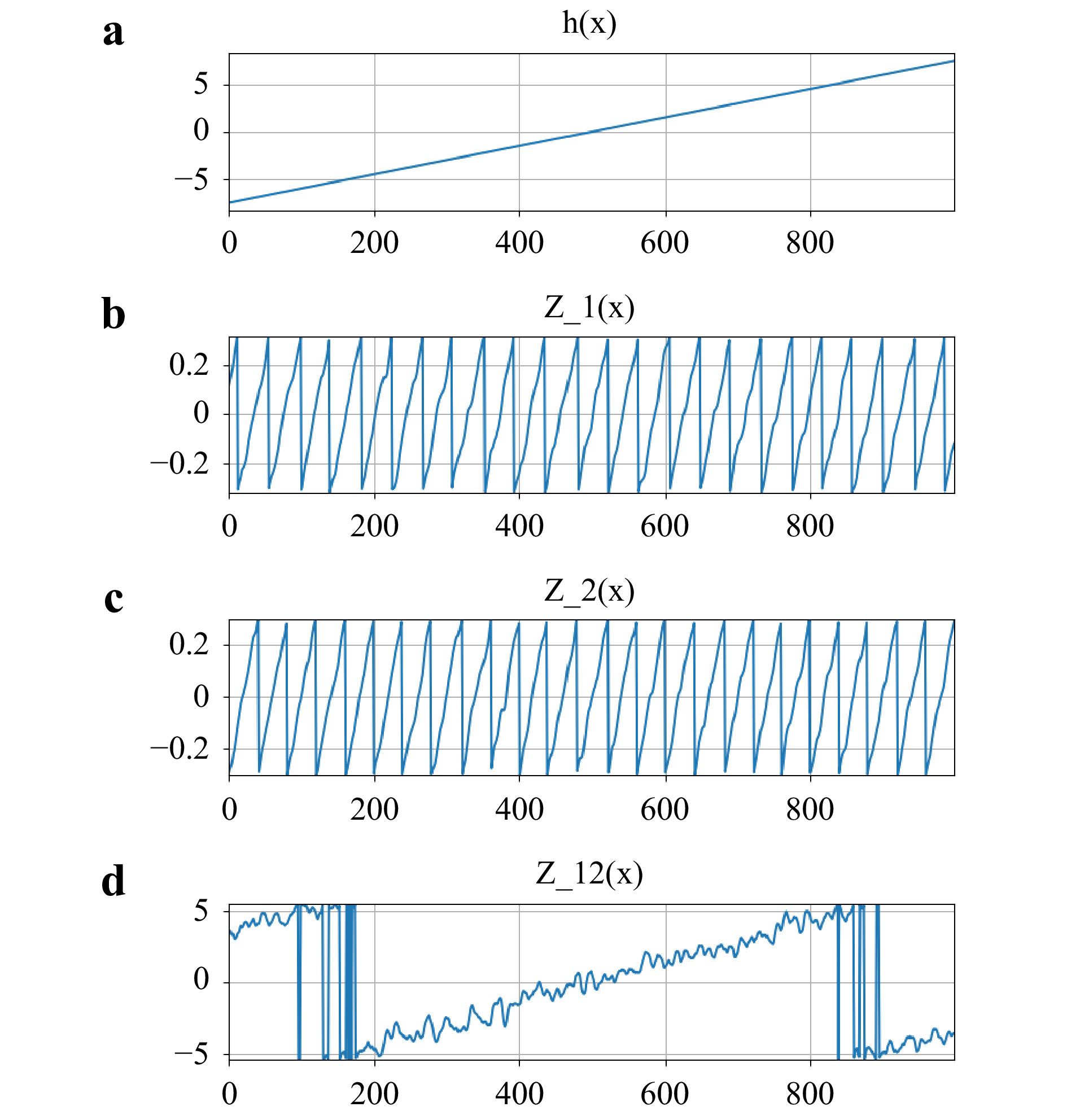

Fig. 11  Simulation of 2-wavelength optical phase unwrapping. a $ h\left(x \right) $; b $ {Z_1}\left(x \right) $; c $ {Z_2}\left(x \right) $; d $ {Z_{12}}\left(x \right) $. The vertical scales are in $ \mu {\rm{m}} $. The horizontal scale is the pixel index. Height of the incline is 15 $ \mu {\rm{m}} $. Assumed wavelengths are $ {\lambda _1} = 0.635 \; \mu {\rm{m}} $, $ {\lambda _2} = 0.600 \; \mu {\rm{m}} $, so that $ {\Lambda _{12}} = 10.886 \; \mu {\rm{m}} $. Phase noise of $ \varepsilon = 3 \%$ results in height noise $ \delta {Z_{12}} = 0.462 \; \mu {\rm{m}} $.

The complex optical fields

are computed from the captured holographic interference patterns, where $ {a_n}\left({x,y} \right) $ and $ {\Phi _n}\left({x,y} \right) $ are the amplitude and phase profiles of the optical field, respectively. In off-axis holography, the phase is encoded as a modulation of the high-spatial-frequency interference fringe patterns in a single camera frame, whereas in phase-shifting digital holography, three or more camera frames are combined while the phase of reference field is shifted. If the acquired optical field resulted from reflection from or transmission through a structured surface or layer, the phase profile $ {\Phi _n}\left({x,y} \right) $ is directly proportional to the profile of the optical path length $ Z\left({x,y} \right) $

The wrapped phase problem arises from the fact that the optical phase is defined only up to modulo $ 2\pi $, and the derived surface height profile

is limited to modulo $ {\lambda _n} $. In Fig. 11b the height profile $ {Z_1} $ acquired using a wavelength $ {\lambda _1} = 0.635 \; \mu {\rm{m}} $ has a sawtooth shape of height equal to the wavelength. A phase noise of standard deviation $ 2\pi \cdot \varepsilon $, with $ \varepsilon = 3\% $, is added in the phase profile to simulate random phase noise between hologram acquisitions.

Two-wavelength optical phase unwrapping is based on taking the conjugate product of two optical fields acquired with two slightly different wavelengths, $ {\lambda _1} $ and $ {\lambda _2} $, as

where

The particular modulo operation is necessary when the phase angle of a complex number is defined in the range $ \left[ { - \pi,\pi } \right] $. The difference phase $ {\Phi _{12}} $ is equivalent to the phase of an effective, or synthetic, wavelength $ {\Lambda _{12}} $, which can be much larger than the original wavelengths:

where

The optical path derived from the difference phase can range up to the synthetic wavelength,

as illustrated in Fig. 11d with $ {\lambda _1} = 0.635\;0 \;\mu {\rm{m}} $ and $ {\lambda _2} = 0.600\;0 \; \mu {\rm{m}} $, so that $ {\Lambda _{12}} = 10.886 \;\mu {\rm{m}} $, and the height profile $ h\left(x \right) $ is properly represented up to the maximum $ {\Lambda _{12}} $.

By choosing two closely spaced wavelengths $ {\lambda _1} $ and $ {\lambda _2} $, the synthetic wavelength $ {\Lambda _{12}} $ can be made as large as necessary to cover the maximum surface height of the object to be profiled. On the other hand, the extension of the synthetic wavelength comes with amplification of noise in the height profile. For suppose the phase noise in $ {\Phi _1} $ is a fraction of $ 2\pi $,

where ε is a dimensionless random function that includes both spatial and frame-to-frame variations. The corresponding noise in the derived optical path is

which is approximately $ \delta {Z_1} = 0.019\; \mu {\rm{m}} $ with the assumed values of $ {\lambda _1} = 0.635 \; \mu {\rm{m}} $ and $ \varepsilon = 3\%$. The noise in the optical height derived from the difference phase and synthetic wavelength is, with $ \delta {\Phi _{12}} \approx \sqrt 2 \delta {\Phi _1} $,

and the noise in the optical height is amplified in proportion to the amplification in wavelength, to approx. $ \delta {Z_{12}} \approx 0.462\;\mu {\rm{m}} $ in Fig. 11d. The amplification in wavelength is accompanied by similar amplification in noise.

The noise can be reduced if a shorter synthetic wavelength, $ {\Lambda _{13}} $ is used, with a larger difference $ {\lambda _1} - {\lambda _3} $. The simulation in Fig. 12 uses $ {\lambda _3} = 0.530\;0\; \mu {\rm{m}} $, so that $ {\Lambda _{13}} = 3.205 \; \mu {\rm{m}} $. Start from $ {Z_{12}}\left({x,y} \right) $ with the range $ {\Lambda _{12}} = 10.886 \; \mu {\rm{m}} $, Fig. 12a, and make integer steps of $ {\Lambda _{13}} $, Fig. 12b. Then, ‘stitch’ the steps with the new profile $ {Z_{13}}\left({x,y} \right) $, Fig. 12c. That is,

Fig. 12  Simulation of 3-wavelength optical phase unwrapping. a $ {Z_{12}} $; b $ {Y_{12}} = {\rm{round}}\left( {{Z_{12}}/{\Lambda _{13}}} \right) \cdot {\Lambda _{13}} $; c $ {Z_{13}} $; d $ {Z'_{12 \cdots 3}} = {Y_{12}} + {Z_{13}} $; e $ {Z_{12 \cdots 3}} $. The vertical scales are in $ \mu {\rm{m}} $. The horizontal scale is the pixel index. Assumed third wavelength is $ {\lambda _3} = 0.530 \; \mu {\rm{m}} $, so that $ {\Lambda _{13}} = 3.205 \; \mu {\rm{m}} $. Final height noise is reduced to $ \delta {Z_{12 \cdots 3}} = 0.136 \; \mu {\rm{m}} $.

where $ {\rm{round}}\left({} \right) $ represents integer rounding operation. If the phase noise is included in the above expression,

Here $ \Delta \cdot {\Lambda _{13}} $ represents spikes of height $ {\Lambda _{13}} $ scattered at positions near the step boundaries of $ {\rm{round}}\left({} \right) $, as evident in Fig. 12d. These spikes can be suppressed by adding or subtracting $ {\Lambda _{13}} $ wherever the absolute difference $ \left| {{Z_{12}} - {Z_{12 \cdots 3}}} \right| $ is comparable to $ {\Lambda _{13}} $. This process is valid with the requirement

and $ {\Lambda _{13}} $ should be chosen large enough compared to $ \sqrt 2 \varepsilon \cdot {\Lambda _{12}} $, or

The overall noise is then reduced from $ \sqrt 2 \varepsilon \cdot {\Lambda _{12}} \approx $$ 0.462\; \mu {\rm{m}} $ to $ \sqrt 2 \varepsilon \cdot {\Lambda _{13}} \approx 0.136 \; \mu {\rm{m}} $, as demonstrated in Fig. 12e.

In the above simulation example, the synthetic wavelength is extended to over 10 $ \mu {\rm{m}} $, which can be suitable for profiling microscopically structured surfaces. On the other hand, for applications requiring profiling of macroscopic surfaces with millimeters of height range, the large amplification of wavelength entails similarly large noise. In order to reduce the large noise, it is then necessary to extend the iterative series using a larger number of wavelengths. Thus, another difference phase profile $ {\Phi _{14}}\left({x,y} \right) $ with synthetic wavelength $ {\Lambda _{14}} < {\Lambda _{13}} $ is used to ‘stitch’ the new profile $ {Z_{14}}\left({x,y} \right) $ on to the previous synthesized profile $ {Z_{12 \cdots 3}}\left({x,y} \right) $. If we again let $ {\Lambda _{14}} = \alpha {\Lambda _{13}} $, the noise level for the new profile $ {Z_{12 \cdots 4}} $ is $ \delta {Z_{12 \cdots 4}} = \sqrt 2 \varepsilon {\Lambda _{14}} = \sqrt 2 \varepsilon \cdot {\alpha ^2}{\Lambda _{12}} $. The process can continue until $ \delta {Z_{12 \cdots n}} = \varepsilon \cdot {\Lambda _{1n}} = \varepsilon \cdot {\alpha ^{\left({n - 2} \right)}}{\Lambda _{12}} $ reaches desired height resolution. In the simulation of Fig. 13, the height range is now $ {\Lambda _{12}} = 2\; 000.0 \; \mu {\rm{m}} $ with $ {\lambda _1} = 0.635\; 000 \; \mu {\rm{m}} $ and $ {\lambda _2} = 0.634\; 798 \; \mu {\rm{m}} $, or $ {\Delta _{12}} = {\lambda _1} - {\lambda _2} = 0.000 \;202 \; \mu {\rm{m}} $. Three more wavelengths are used with difference wavelengths $ {\Delta _{13}} = 0.000\; 805 \; \mu {\rm{m}} $, $ {\Delta _{14}} = 0.003\; 209\; \mu {\rm{m}} $, and $ {\Delta _{15}} = 0.012\; 646 \; \mu {\rm{m}} $ for synthetic wavelengths $ {\Lambda _{13}} = 500.0 \; \mu {\rm{m}} $, $ {\Lambda _{14}} = 125.0\; \mu {\rm{m}} $, and $ {\Lambda _{15}} = 31.25 \; \mu {\rm{m}} $, respectively, with a fixed stepping factor $ \alpha = 0.25$ for the series. Assuming phase noise with $ \varepsilon = 3\%$, the initial noise 84.9 $ \mu {\rm{m}} $ in $ {Z_{12}} $ is progressively reduced to 21.2 $ \mu {\rm{m}} $, 5.3 $ \mu {\rm{m}} $, and 1.3 $ \mu {\rm{m}} $ in $ {Z_{13}} $, $ {Z_{14}} $, and $ {Z_{15}} $, respectively.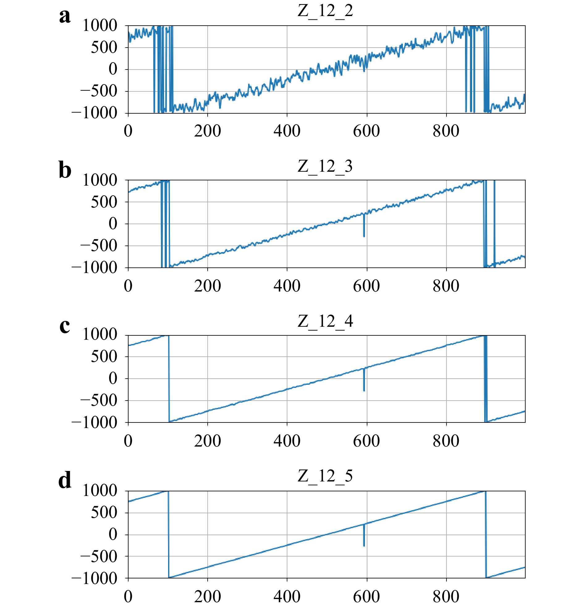

Fig. 13  Simulation of iterative reduction of noise for large height range $ {\Lambda _{12}} = 2 000.0 \; \mu {\rm{m}} $, using a series of five wavelengths. a $ {Z_{12}}\left(x \right) $; b $ {Z_{12 \cdots 3}}\left(x \right) $; c $ {Z_{12 \cdots 4}}\left(x \right) $; d $ {Z_{12 \cdots 5}}\left(x \right) $. The vertical scales are in $ \mu {\rm{m}} $. The horizontal scale is the pixel index. With a stepping factor $ \alpha = 0.25 $, the synthetic wavlengths are set to $ {\Lambda _{1n}} = [2\; 000.0, $$ 500.0, 125.0, 31.25] \; \mu {\rm{m}} $, for $ n = 2,\, \cdots,\,5 $, which can be obtained from the wavelengths $ {\lambda _n} = [0.635\; 000, 0.634\; 798, 0.634\;195, 0.631\;791, $$ 0.62\; 354] \; \mu {\rm{m}} $, for $ n = 1,\,2,\, \cdots,\,5 $. With the assumed phase noise of $ \varepsilon = 3\% $, the height noise progressively dcreases as $ \delta {Z_{12 \cdots n}} = [77.7, 20.5, 5.3, 1.2] \; \mu {\rm{m}} $ for $ n = 2,\, \cdots,\,5 $.

If the iteration is made to run too fast with the stepping factor α too small, the noise reduction by stitching as described above can be incomplete and significant amount of noise can remain after the procedure. In Fig. 14a, the noise is increased to $ \varepsilon = 7\%$ while using the same set of wavelengths $ {\lambda _1}, \cdots,{\lambda _5} $, with $ \alpha = 0.25$, as the above example. The condition $ \varepsilon \ll \alpha $ is not sufficiently strong that there are many spikes $ \Delta \cdot {\Lambda _{1n}} $ in resulting profiles $ {Z_{12 \cdots n}} $. In order to improve the noise figure, we slow the iteration using a larger value of $ \alpha = 0.50$, and increase the number of wavelengths to eight, so that the final synthetic wavlengths in the two series are the same: $ {\Lambda _{18}} = 31.25 \; \mu {\rm{m}} $ with $ \alpha = 0.25$ and $ {\Lambda _{15}} = 31.25 \; \mu {\rm{m}} $ with $ \alpha = 0.50$. In Fig. 14b, the stitching process is applied to the series of eight wavelengths to obtain the profiles $ {Z_{12}},\,{Z_{12 \cdots 3}},\, \cdots, $$ \,{Z_{12 \cdots 8}} $. The final noise level close to $ \delta {Z_{12 \cdots 8}} = 2.19 \;\mu {\rm{m}} $ is achieved without significant number of spike. This simulation result suggests that large height or noisy surfaces may be profiled using slower progression of $ {\Lambda _{1n}} $, i.e. larger α, and larger number of wavelengths.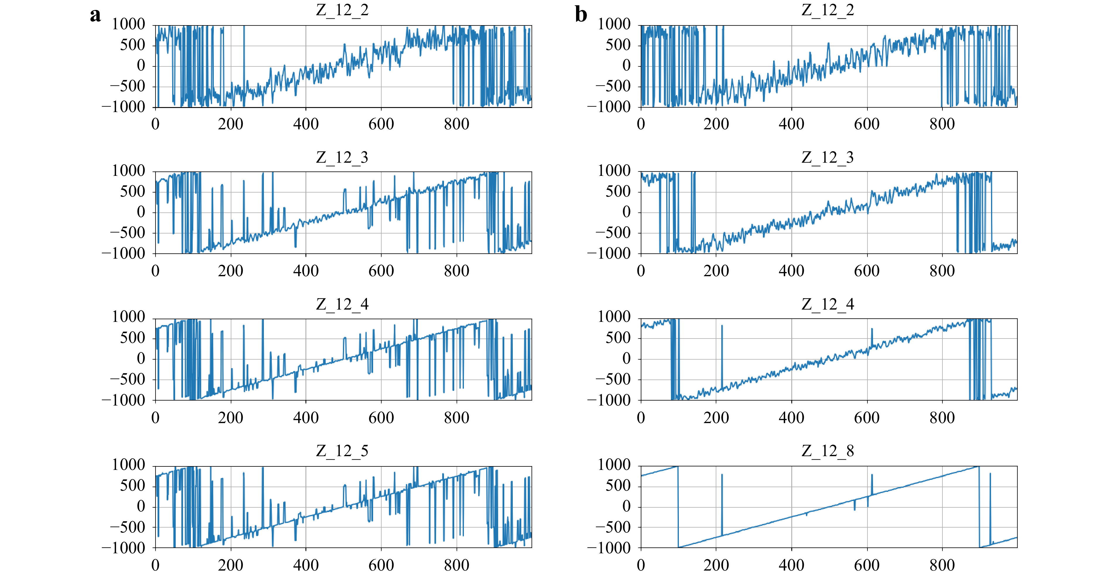

Fig. 14  Effect of stepping factor α for large noise profiles, with $ \varepsilon = 7\% $. For the column a, the same stepping factor $ \alpha = 0.25 $ is used as in Fig. 13. The measured height noise is $ \delta {Z_{12 \cdots n}} = [110.0, 37.2, 51.6, 50.6] \; \mu {\rm{m}} $ for $ n = 2,\, \cdots,\,5 $. For the column b, a slower stepping factor $ \alpha = 0.50 $ is used with eight wavelengths, so that the final synthetic wavelength $ {\Lambda _{18}} = 31.25 \; \mu {\rm{m}} $ is the same as $ {\Lambda _{15}} $ in a). Graphs for $ {Z_{12 \cdots 5}} \sim{Z_{12 \cdots 7}} $ are omitted. The vertical scales are in $ \mu {\rm{m}} $. The horizontal scale is the pixel index. Now, the measured height noise is $ \delta {Z_{12 \cdots n}} = [99.2, 51.5, 35.5, $$ 13.8, 11.5, 2.9, 2.2] \; \mu {\rm{m}} $ for $ n = 2,\, \cdots,\,8 $. That is, the final noise value of $ \delta {Z_{12 \cdots 8}} = 2.2\,\mu {\rm{m}} $ obtains for $ \alpha = 0.50 $, instead of $ \delta {Z_{12 \cdots 5}} = 50.6\,\mu {\rm{m}} $ for $ \alpha = 0.25 $.

The ‘stitching’ process is rather sensative to a few different types of errors and these need to be addressed carefully. The process requires that each of the phase profiles $ {\Phi _n}\left({x,y} \right) $ is referenced to an identical global phase, which is never the case due to random variations in the laser, optical, and mechanical systems. This is remedied by fixing the difference phase $ {\Phi _{1n}}\left({{x_0},{y_0}} \right) $ at a suitable, relatively noise-free, reference point to be zero.

Another source of error is that the synthetic wavelength is inversely proportionale to a small difference wavelength. In MWDH, the laser wavelengths drift with temperature and other factors. Although a high precision wave meter is available, the current setup does not incorporate tight monitoring and control of it. In MADH, the angular position is more closely monitored but the precision is limited and any mechanical instability may affect it. In any case, at least in the current setup, it is necessary, during post-processing, to verify and adjust the accuracy of synthetic wavelengths. This is carried out by scanning the synthetic wavelength over a range and looking for optimal values for minimizing the noise spikes.

For example, to achieve a height range of $ {\Lambda _{12}} = 2.0$ mm near $ \lambda = 0.635\;\mu {\rm{m}} $, the required wavelength difference is $ \Delta \lambda \approx 0.2$ nm. And to achieve $ \mu {\rm{m}} $ -level height resolution, several wavelengths are needed. For such applications, acquiring and maintaining multiple laser sources with precision-tuned wavelengths quickly becomes prohibitively difficult. The cost and complexity of the optical system can be significantly reduced if, instead of multiple lasers, a single laser is used and the multiple effective wavelengths are generated by changing the illumination angle of the object. The variation of the optical phase through a given height h of the object is $ 2\pi h/\lambda \cos \theta $, which can be described as illumination from a fixed direction with effective wavelength

Multiple effective wavelengths $ {\lambda _n} $ can be generated simply by tuning the illumination angle to various positions $ {\theta _n} $. The synthetic wavelength between the 1st and n-th effective wavelengths is then

The rest of the theoretical description of MADH is in exact parallel with that of MWDH, but there are significant differences in practical considerations of the two methods. The MWDH requires multiple lasers or tunable lasers as well as a means to combine and switch between them, whereas the MADH requires one good laser and a means for fine control of illumination angle. To achieve 2.0 mm height range as above, the required angle shift is $ \Delta \theta = {0.070^ \circ } $, when $ \theta = {15^ \circ } $, indicating the level of angular precision needed. The MADH is mostly immune from chromatic aberration but can be affected by spherical or higher order geometric aberrations due to the movement of the illumination across optical apertures. In order to keep $ {\Lambda _{1n}} $ becoming too large, or the angular step $ \Delta \theta $ too small, the angle θ needs to be somewhat away from zero, $ \theta \sim {15^ \circ } $ for example. This can cause shadowing or obscuration of the object surface when the surface has sharp or tall features.

A schematic of one version of the optical system is depicted in Fig. 15, based on Michelson interferometer configuration. It can accommodate several operating modes, including multi-wavelength or multi-angle holography, as well as off-axis or phase-shifting holography. The fiber coupler FC introduces laser light into the system. Typical power input at FC is a few mW. Expanded and collimated beam is reflected by the mirror MI. The confocal lens combination L1 (f1 = 100 mm) and L2 (f2 = 200 mm) images the rotating mirror to the object plane, which is in turn imaged on to the camera plane by the lens L4 and a camera lens LC. The reference mirror MR is also conjugate with the camera plane, and is mounted on a piezo actuator for phase shifting. The polarizing beam-splitter PBS and quarter wave plates QO and QR together with the polarizer P controls and optimizes intensity ratio between the object and reference beams. The lenses L2 and L4 and quarter wave plates and polarizer, as well as the polarizing beam splitter are 2 inches in diameter or width. Typical field of view of the object plane is 10 ~ 30 mm.

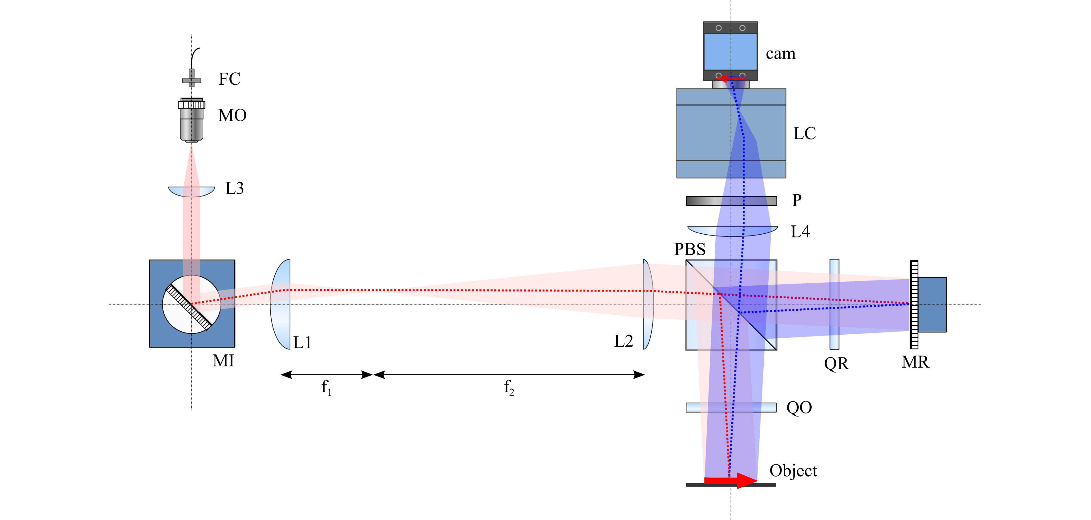
Fig. 15  Schematic of the MWDH/MADH apparatus. FC: fiber coupler; MO: microscope objective; L3: collimating lens; MI: illumination mirror on digital rotation stage; L1 & L2: confocal lens pair to image MI to object and reference planes; PBS: polarizing beam splitter; QO & QR: quarter wave plates; MR: piezo-mounted reference mirror; L4 & LC: camera imaging lens; P: linear polarizer; cam: camera.

For multi-wavelength experiments, a set of four lasers (Lasos DPSS) are used with nominal wavelengths $ {\lambda _1} = 639.617$ nm, $ {\lambda _2} = 639.592$ nm, $ {\lambda _3} = 639.416$ nm, and $ {\lambda _4} = 637.928$ nm. These lasers are fiber-coupled into a four-channel fiber switch (Leoni), before being coupled into the interferometer. All fibers are polarization preserving single mode. The laser wavelengths do drift with changing temperature, and a high finesse wavemeter (Toptica) with 0.1 pm resolution was used to measure the wavelengths in real time before calculating synthetic wavelengths and other parameters.

For multi-angle experiments, a 30 mW HeNe laser fiber-coupled into the interferometer is deflected by the illumination mirror MI mounted on a motorized rotation stage (Thorlabs DDR25), which has encoder resolution of 0.00025 deg/count. The starting angle $ {\theta _0} = {18^\circ } $ is set with manual estimate using a ruler. Instead of trying to measure this angle with any better precision, the synthetic wavelength can be calibrated according to the known step size of an object. By placing both the object and reference planes conjugate to the camera, it is ensured that the relative angle of incidence between the two beams does not change with the rotation of the mirror.

In another configuration, based on a modified Mach-Zhender interferometer, only the object beam is tilted while the reference beam remains stationary. This produces a slope in the holographic phase profile, but can be easily compensated for numerically in reconstruction. The reference mirror MR can be tilted by an appropriate amount for off-axis digital holography, or piezo-shifted for phase-shifting digital holography.

Typically, a complex-valued hologram is acquired by combining several camera frames of interference intensity while the reference mirror is piezo-shifted, per standard procedures of phase-shifting digital holography. Then the source wavelength is switched in MWDH or the MI mirror angle is switched in MADH. A series of such holograms are acquired, which are then post-processed to construct the 3D surface profile of the object. Python-based programs are used for most of hardware control, image acquisition, and holographic image processing. Some parts of the software system also use LabVIEW and Matlab.

This project has not been externally funded.