


HTML
-
The phase of an optical field contains various sources of information. Holography, invented by Gabor in 19471, provides access to phase information and has been used as a powerful imaging technique2,3. At the optical frequency, however, electromagnetic waves oscillate so fast that the detection devices can directly record only the average incident power. The loss of phase information poses unique challenges for the numerical inversion of the imaging process, leading to the so-called “twin-image” effect that severely degrades the imaging quality4,5. As a result, phase retrieval, or the recovery of the phase from intensity-only measurements, remains a longstanding issue and lies at the heart of digital holography and many related optical imaging techniques6. In recent years, phase retrieval has regained increasing research interests following the development of computational imaging, which leverages advancements in signal processing theory, numerical algorithms, hardware design, and computation power7.
Existing phase retrieval methods for in-line holography can be broadly classified into two categories, namely diversity phase retrieval and compressive phase retrieval. The former approach requires taking multiple images with some data diversity that translate phase information into intensity distribution. This can be achieved, for example, by varying the imaging distance8−10, illumination wavelength11−14, probe position15−17, illumination angle18−20, and modulation pattern21−24. While this approach can achieve quantitative phase imaging with increased data diversity and redundancy, it sacrifices the temporal resolution, system cost, and complexity. As an alternative, compressive phase retrieval takes a different path by exploring additional prior knowledge of the wavefield, which could potentially achieve phase recovery beyond the information-theoretic limit or even from a single shot.
Historically, early works tackled the phase ambiguity problem by utilizing simple yet effective physical constraints such as non-negativity25,26, support27−29, absorption30, histogram31, and atomicity32. These constraints are typically enforced via projections in the complex Euclidean space, and the corresponding phase retrieval algorithms proceed by projecting the estimated wavefield back in an iterative manner33,34. Since the seminal Gerchberg-Saxton35 and Fienup’s error-reduction algorithms36, iterative projection algorithms have played a pivotal role in phase retrieval for decades37−39. However, this classical approach relies on carefully handcrafted physical constraints, which may fail to fully extract the inherent features of complex scenes under limited measurements, particularly in the case of single-shot phase retrieval40. Consequently, it has mostly been demonstrated for simple objects. The quantitative phase analysis of complex samples, such as dense biological specimens, remains a challenging task.
The concept of compressive phase retrieval was formally established by an explosion of theoretical and empirical studies following the development of compressed sensing41−43. Sparsity priors in various domains such as the spatial44−49, gradient50−61, wavelet62 and other domains63,64 or with a dictionary-learned transform65−67 have been demonstrated as effective regularizers for phase recovery. More recently, implicit image priors from advanced denoisers such as BM3D68−73 or represented by deep neural networks74−93 have also been studied in the context of phase retrieval, resulting in improved reconstruction quality. Although the regularization techniques generally yield superior imaging performance, they are highly dependent on the scene and may require manual fine-tuning to achieve satisfactory results.
In pursuit of a compressive phase retrieval method for in-line holography that features both robustness and high fidelity, we propose a novel computational framework that encapsulates physical constraints and sparsity priors as a unified optimization problem. Specifically, we consider the well-known absorption and support constraints and gradient-domain sparsity, leading to a constrained complex total variation (CCTV) model. This is because TV-regularized problems can be solved using computationally efficient algorithms and are thus highly scalable to large-scale problems94,95. The piece-wise smoothness underlying the TV model can also characterize multidimensional data such as the three-dimensional refractive index distribution, offering good generalizability to various applications96−99. Furthermore, TV-regularized inversion algorithms offer mathematically tractable convergence behaviors, which is important for both theoretical soundness and practical implementation.
Based on the CCTV model, compressive phase retrieval is formulated as a regularized inverse problem and is solved via an accelerated proximal gradient algorithm together with an efficient denoiser for the proximal update. Unlike conventional methods that rely on a heuristic basis, we provide a rigorous mathematical analysis that guarantees the convergence of the proposed algorithms using prespecified parameters. We experimentally demonstrated quantitative phase imaging of various samples from a single in-line hologram, illustrating the effectiveness of the CCTV model in characterizing complex real-world scenes while leveraging physically tractable constraints for quality enhancement. We further elaborate on algorithmic behaviors based on extensive numerical studies, corroborating the theoretical results while providing general guidance for practitioners.
-
For electromagnetic waves at optical frequencies, sensors can only respond to the average power of the incident wavefield. Thus, phase information, i.e., the complex argument of the signal, is lost during the measurement process. The forward model can be abstractly expressed, regardless of the imaging configuration, in a vectorized form as
$$ {\boldsymbol{y}} = |{\boldsymbol{Ax}}| $$ (1) where
$ {\boldsymbol{y}}\in\mathbb{R}^m $ is the observed measurement,$ {\boldsymbol{A}}\in\mathbb{C}^{m\times n} $ is the sampling matrix, and$ {\boldsymbol{x}}\in\mathbb{C}^n $ is the underlying complex signal that represents the transmission of the object. In the vectorized formulation, column vectors$ {\boldsymbol{x}} $ and$ {\boldsymbol{y}} $ are raster-scanned from the corresponding two-dimensional complex object transmission function and hologram amplitude, respectively. It is important to note that, the purpose of vectorization is to simplify the algorithm derivation and notations. Vectorization is not required when implementing the algorithm in practice.Generally, the sampling matrix may involve various linear physical processes such as probe illumination, free-space propagation and mask modulation, all of which are determined by the optical configuration of the imaging system. In this work, we consider the lensless in-line holographic imaging model for illustration, which is shown in Fig. 1a. The object is illuminated by a coherent plane wave, such that the retrieved complex field directly reveals the absorption and phase shift introduced by the object. An imaging sensor was placed close to the object, and the in-line hologram was recorded. Such a simple optical configuration enables low-cost and portable system design for various imaging applications100,101. The physical process involves only free-space propagation of the wavefield, which is calculated using the angular spectrum method102. Therefore, the sampling matrix of our imaging model can be expressed as
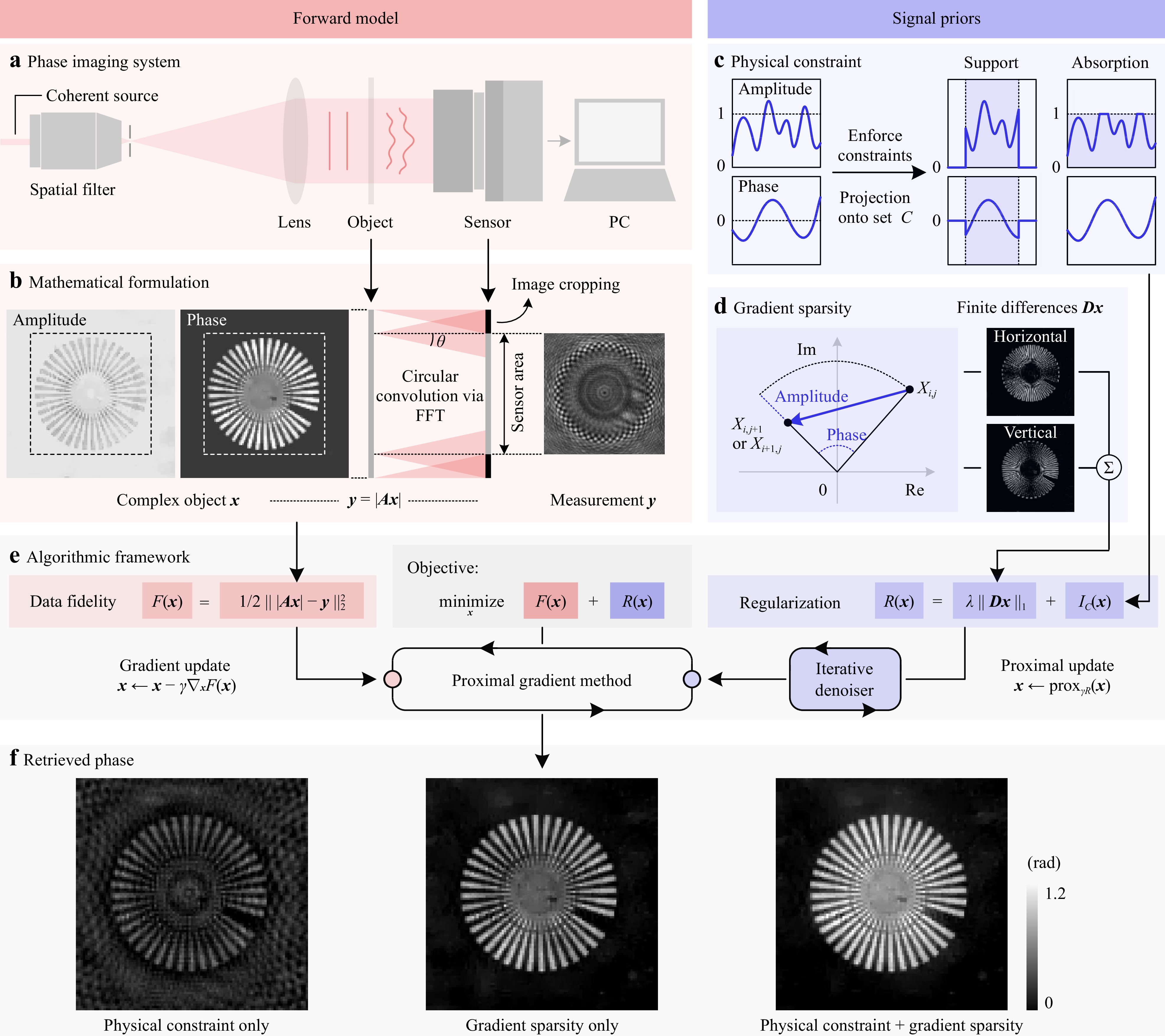
Fig. 1 Schematic of the proposed compressive phase retrieval framework. a The optical configuration of an in-line holographic imaging system. b The angular spectrum diffraction model adopted for numerical calculation. The diffraction angle
$ \theta $ and the corresponding convolution kernel size are determined by the sampling frequency (or, equivalently, the sensor pixel size). c Physical knowledge, such as object support or absorption, is often enforced as hard constraints via projection operations. d The complex TV regularizer promotes sparsity in both the gradients of amplitude and phase. e We combine the forward model and signal priors into an optimization problem, which is solved via the proximal gradient method. An iterative denoiser is introduced for the proximal update step. f Retrieved phase from experimental data. Combining physical constraints and gradient sparsity yields the best performance.$$ {\boldsymbol{A}} = {\boldsymbol{C}} {\boldsymbol{Q}} $$ (2) where
$ {\boldsymbol{Q}}\in \mathbb{C}^{n\times n} $ denotes the free-space propagation operator calculated as a circular convolution with the Fresnel kernel via fast Fourier transforms (FFTs),$ {\boldsymbol{C}}\in\mathbb{R}^{m\times n} $ denotes an image cropping operation to model the finite size of the imaging sensor103. Notice that we have$ m<n $ , that is, the object dimension is larger than the pixel number of the sensor. This is because out-of-field objects may also contribute to the recorded image owing to the linear convolution effect54. This process is illustrated in Fig. 1b.Phase reconstruction from a single in-line hologram is inherently challenging due to the existence of ambiguous solutions. Therefore, compressive phase retrieval takes an inverse problem approach that utilizes regularization techniques to ensure well-posedness. In this work, we introduce the integration of a complex TV and a hard constraint as the regularizer, leading to an optimization problem in the following form:
$$ \mathop{{\rm{min}}}\limits_{{\boldsymbol{x}}} \, \underbrace{\frac{1}{2} \vphantom{\frac{1}{\frac{1}{1}}} \left\| |{\boldsymbol{Ax}}| - {\boldsymbol{y}} \right\|_2^2}_{F({\boldsymbol{x}})} + \underbrace{\lambda \| {\boldsymbol{D}} {\boldsymbol{x}} \|_1 + I_C({\boldsymbol{x}}) \vphantom{\frac{1}{\frac{1}{1}}} }_{R({\boldsymbol{x}})} $$ (3) where
$ \| \cdot \|_p $ denotes the$ \ell_p $ vector norm or the corresponding matrix norm.$ F({\boldsymbol{x}}) $ is the data-fidelity term and$ R({\boldsymbol{x}}) $ is the regularization term. The fidelity term ensures that the solution does not deviate significantly from the forward model in Eq. 1. Meanwhile, the regularization term introduces additional prior knowledge of the wavefield to improve the reconstruction quality further.There are various choices for the fidelity function
$ F({\boldsymbol{x}}) $ in the phase retrieval literature, such as the intensity-based formulation$ F({\boldsymbol{x}}) = (1/2) \| |{\boldsymbol{Ax}}|^2 - {\boldsymbol{y}}^2 \|_2^2 $ 104−106 and the amplitude-based formulation$ F({\boldsymbol{x}}) = (1/2) \| |{\boldsymbol{Ax}}| - {\boldsymbol{y}} \|_2^2 $ 107−109. The main reasons for choosing the amplitude-based residual here are threefold. First, from a physical perspective, it is closely related to the maximum likelihood estimation under Poisson noise, which captures the noise statistics more accurately than the Gaussian noise model110. Second, on the practitioner’s side, using the amplitude-based formulation ensures the convergence of the iterative algorithms with a prespecified algorithm step size, obviating the need for complicated line searches and simplifying the implementation. Third, many empirical studies have observed faster convergence when minimizing amplitude-based fidelity functions111,112.The proposed regularization function
$ R({\boldsymbol{x}}) $ comprises two separate terms. The first term is the sparsity regularizer with the parameter$ \lambda > 0 $ . Specifically, we considered the anisotropic complex TV seminorm:$$ \begin{split} \| {\boldsymbol{D}} {\boldsymbol{x}} \|_1 = &{\rm{TV}}({\boldsymbol{X}}) \\ =&\sum\limits_{i=1}^{n_\xi-1} \sum\limits_{j=1}^{n_\upsilon \vphantom{n_\xi}} |X_{i+1,j} - X_{i,j}| + \sum\limits_{i=1}^{n_\xi} \sum_{j=1}^{n_\upsilon - 1 \vphantom{n_\xi}} |X_{i,j+1} - X_{i,j}| \end{split} $$ (4) where
$ {\boldsymbol{X}}\in\mathbb{C}^{n_\xi \times n_\upsilon} $ with$ n_\xi n_\upsilon = n $ denotes the non-vectorized two-dimensional image corresponding to$ {\boldsymbol{x}} $ .$ {\boldsymbol{D}} \in \mathbb{C}^{2n\times n} $ denotes the spatial finite-difference operator for the vectorized$ {\boldsymbol{x}} $ along the two directions. As shown in Fig. 1d, the complex TV reveals both the amplitude and phase variations between adjacent sampling points of the object transmission function and thus serves as a good sparsifying transform for complex-valued images113. Apart from the complex TV, we introduce a second regularizer$ I_C({\boldsymbol{x}}) $ , which is an indicator function of the constraint set$ C $ . This is motivated by conventional iterative projection (IP) phase retrieval algorithms, where phase retrieval is formulated as a feasibility problem, and the unknown field distribution is assumed to belong to certain physical constraint sets. The IP algorithms typically proceed by projecting the estimated wavefield onto constraint sets in an iterative manner37,38. Here, we consider the support and absorption constraints in particular because they are commonly adopted for reconstructing complex objects, and their corresponding constraint sets are both convex. Fig. 1c presents a conceptual illustration of these physical constraints, and the mathematical definitions are presented in Table 1. The proposed regularizer$ R({\boldsymbol{x}}) $ comprises a complex TV and a hard physical constraint and is thus termed the constrained complex total variation regularizer. As a special case, when$ C=\mathbb{C}^n $ , CCTV reduces to the complex TV function without physical constraints, and when$ \lambda = 0 $ , it reduces to the classical problem of phase retrieval from a modulus measurement and a physical constraint.Constraint Definition of C Projection ${\boldsymbol{x}'}=\mathcal{P}_C(\boldsymbol{x})$ Support ${\boldsymbol{x}}\odot{\bf{1}}_P = {\bf{0}}$ $ x_i^{\prime}= \left\{ {\begin{array}{*{20}{l}}{0,}&{i \in P}\\{{x_i},}&{i \notin P}\end{array}} \right.$ Absorption $|{\boldsymbol{x}}| \leq {\bf{1}}$ $x_i^{\prime} =\left\{ {\begin{array}{*{20}{l}}{{x_i}/\left| {{x_i}} \right|,}&{\left| {{x_i}} \right| > 1}\\{{x_i},}&{\left| {{x_i}} \right| \le 1}\end{array}} \right.$ 1 The symbol $\odot$ denotes the element-wise (Hadamard) multiplication operator. 0 and 1 denote the zero vector and all-ones vector, respectively. P denotes the set of pixels outside the support region, and 1P denotes the indicator vector of P. Table 1. Physical constraints for phase retrieval
-
We built a proof-of-principle in-line holographic imaging system for optical experiments, as shown in Fig. 2a. A 660 nm diode-pumped solid-state laser (Cobolt Flamenco 300) was used as the source for coherent illumination. The optical beam generated by the laser passes through a spatial filter that comprises an objective lens and a pinhole at the back focal plane. The filtered wave was then collimated using a convex lens to illuminate the object. The diffraction pattern was recorded using a CMOS sensor (QHY174GPS, pixel size 5.86 μm, resolution 1920×1200) which was placed a few millimeters away from the object. The captured raw intensity image was then digitally processed using a personal computer for holographic reconstruction. In all optical experiments, we consider only the absorption constraint because the objects have extended field distributions and thus the support constraint is inapplicable. Before running the iterative phase retrieval algorithm, a preprocessing step is required to determine the imaging distance, which can be achieved by either manual tuning or using some autofocusing algorithms114−116. Each captured intensity image is normalized by the background image which is obtained using the same experimental conditions, only with the object removed. This calibration process ensures the validity of the absorption constraint39.
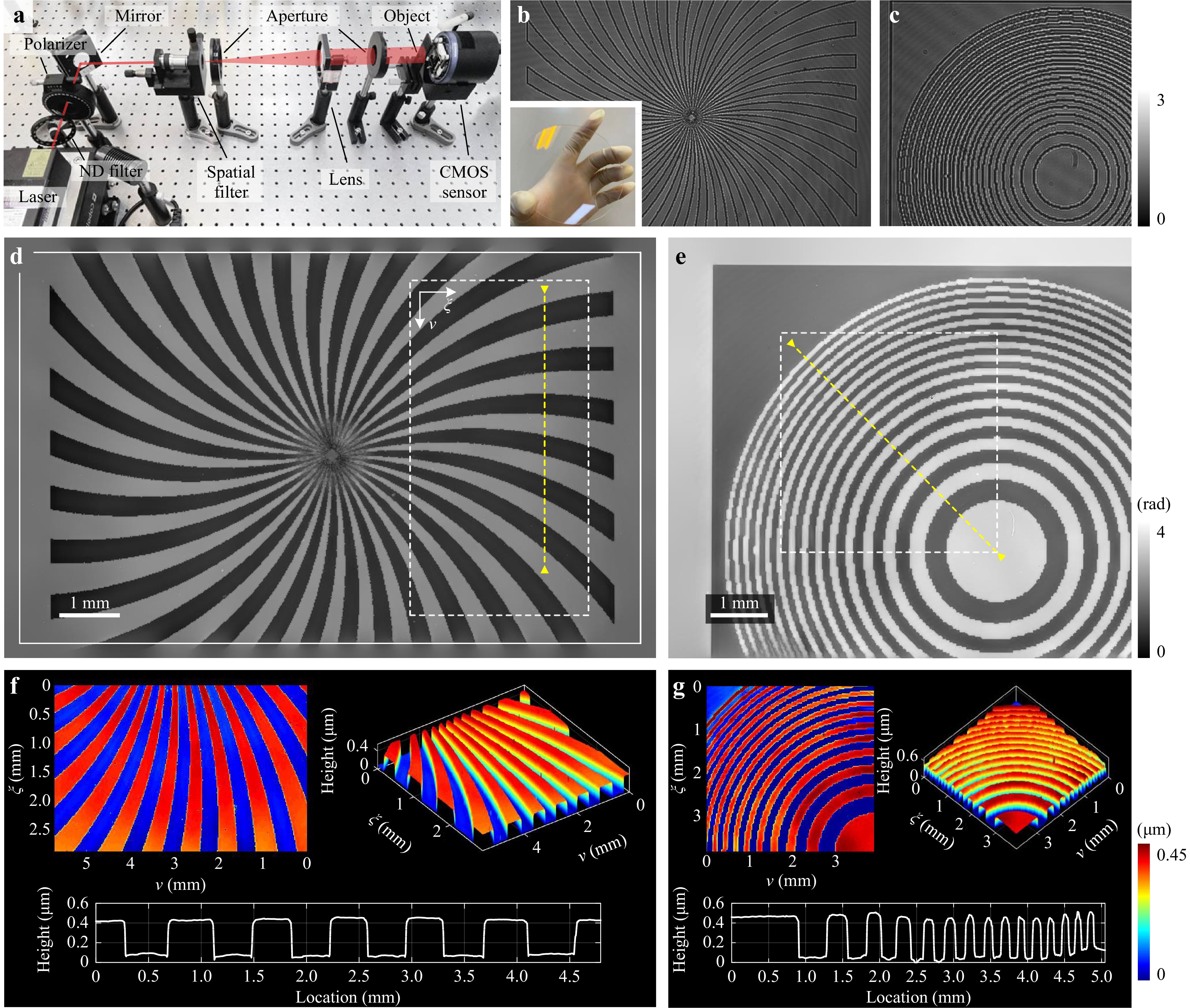
Fig. 2 Experimental characterization of a fabricated phase plate. a Optical setup of the in-line holographic imaging system. b and c show the captured in-line holograms of two transparent patterns. The inset shows an image of the phase plate. d and e show the reconstructed phase distribution from b and c, respectively. The white solid rectangle in d indicates the sensor’s field of view. f and g visualize the rendered surface profiles and the cross-sectional height profiles of d and e, respectively. The white dashed rectangles indicate the enlarged areas, and the yellow dashed lines indicate the cross-sections. The same applies to other figures.
We demonstrated the quantitative phase imaging capability of the proposed compressive phase retrieval method for real-world objects. Fig. 2 shows the imaging results of a phase plate, which was fabricated by etching multiple self-designed binary patterns onto a JGS1 quartz glass substrate. The retrieved phases of the spiral pattern and Fresnel zone plate are shown in Fig. 2d, e, respectively. Smooth staircase profiles with sharp edges can be accurately retrieved. Artifacts on the surface were preserved, indicating a high spatial resolution. Given that the object has a uniform refractive index distribution and that the fabricated features lie only on the surface of the substrate, the surface profiles can be directly calculated and characterized with knowledge of the medium refractive index, as shown in Fig. 2f, g. It is important to note that recovering the low-frequency phase is inherently challenging for the in-line configuration because the weak phase transfer function diminishes to zero together with the spatial frequency117. Hence, slowly varying phase structures hardly contribute to the intensity variations at the sensor plane, rendering them particularly difficult to recover. This has been the main drawback for in-line holography compared to off-axis holography118,119. Our findings suggest that the CCTV regularizer may be a competitive solution for this problem. In addition, because we have addressed the issue of the circular convolution model, the retrieved image is free from boundary artifacts, and the object distribution outside the sensor area can be partially recovered, as shown in Fig. 2d.
We imaged a muscle tissue section to validate the proposed method on complex objects, as shown in Fig. 3. The twin image was effectively eliminated from the retrieved amplitude and phase, which visually demonstrated the high-fidelity imaging performance of the method. The retrieved phase reveals thickness variations inside the tissue slice, facilitating label-free and low-cost clinical studies or diagnoses120,121.
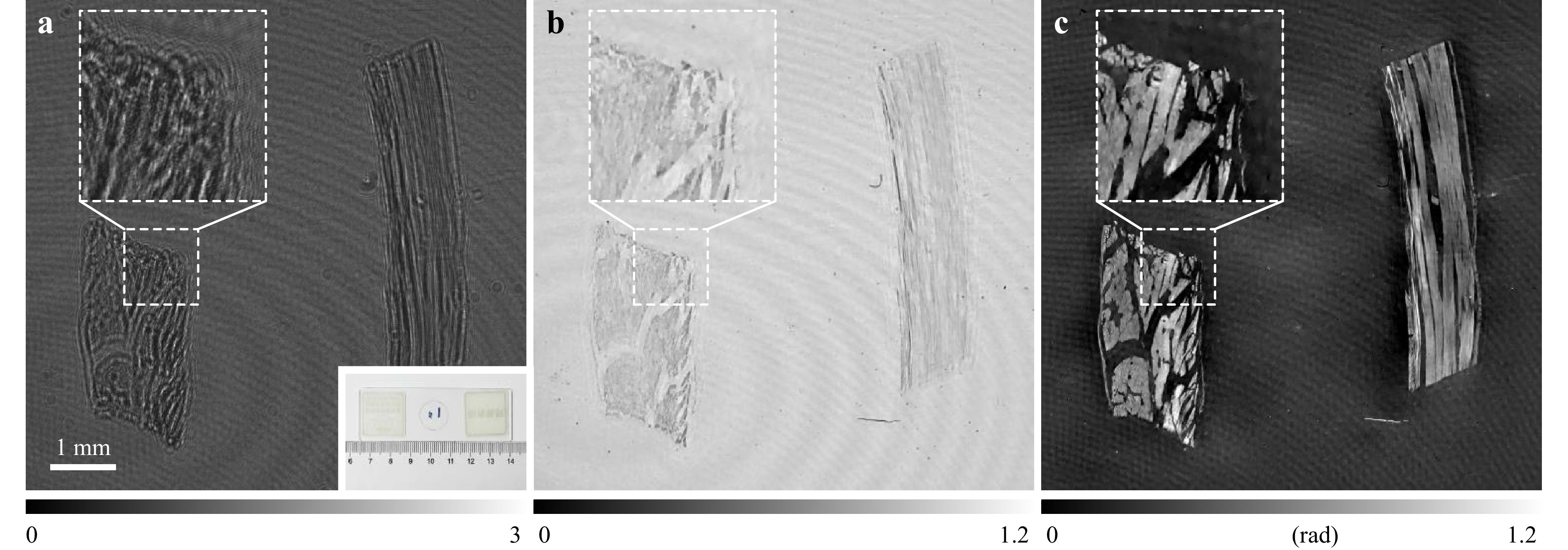
Fig. 3 Holographic imaging results of a muscle tissue section. a Experimentally recorded intensity image. The inset is an image of the sample slide. b and c are the retrieved amplitude and phase, respectively.
-
We conducted ablation studies based on experimental data to quantify the performance improvements obtained by the physical constraints and the complex TV regularizer respectively. For comparison, we implemented compressive phase retrieval algorithms using only physical constraints or gradient sparsity. The former, referred to as the IP method, can be viewed as an accelerated variant of the conventional iterative projection algorithm. This was implemented by setting the regularization parameter
$ \lambda = 0 $ . The algorithm proceeds by iteratively minimizing the data-fidelity function with a gradient descent step and enforcing physical constraints with a projection step. The latter, referred to as the CTV method, uses only the complex TV regularizer without any physical constraints. It is implemented by defining the constraint set$ C=\mathbb{C}^n $ and thus the projection onto set$ C $ is reduced to identity mapping.Both the IP and CCTV methods can utilize various physical constraints. To better differentiate among different methods, we use the letter ‘A’ to represent the method that uses the absorption constraint, the letter ‘S’ for the support constraint, and ‘AS’ for both constraints. For example, ‘IP-A’ represents an iterative projection algorithm that uses only the absorption constraint.
We first performed phase imaging of a quantitative phase microscopy target (Benchmark Technologies) using three methods, namely IP-A, CTV, and CCTV-A, as shown in Fig. 4. Note that the object has an extended distribution and thus the support constraint is inapplicable. The IP algorithm fails to eliminate the twin-image artifact completely, and the phase structures are not clearly revealed, which implies that the physical constraint alone is insufficient to suppress the phase ambiguities. The CCTV method achieved better imaging quality than CTV, as illustrated by visual and quantitative comparisons. The ground-truth phase values were calculated using the structures’ height and medium refractive index, which are both provided by the manufacturer. The root-mean-square errors (RMSEs) of the cross-sectional phase profiles retrieved using the IP-A, CTV, and CCTV-A methods were 0.880, 0.463, and 0.418 rad, respectively. In addition, the finest resolved features of the USAF 1951 resolution target are highlighted. Group 6, Element 3 is resolved by all three methods, indicating a spatial resolution of 80.6 lines/mm, which agrees with the maximum resolution of 85.3 lines/mm of the sensor. All three methods achieve the same sampling-limited resolution, which implies that the TV-based regularizer does not sacrifice the spatial resolution for quality enhancement. The resolution can be further improved beyond the Nyquist sampling limit, however, if one takes into account the down-sampling effect of the sensor pixels112,122−126.
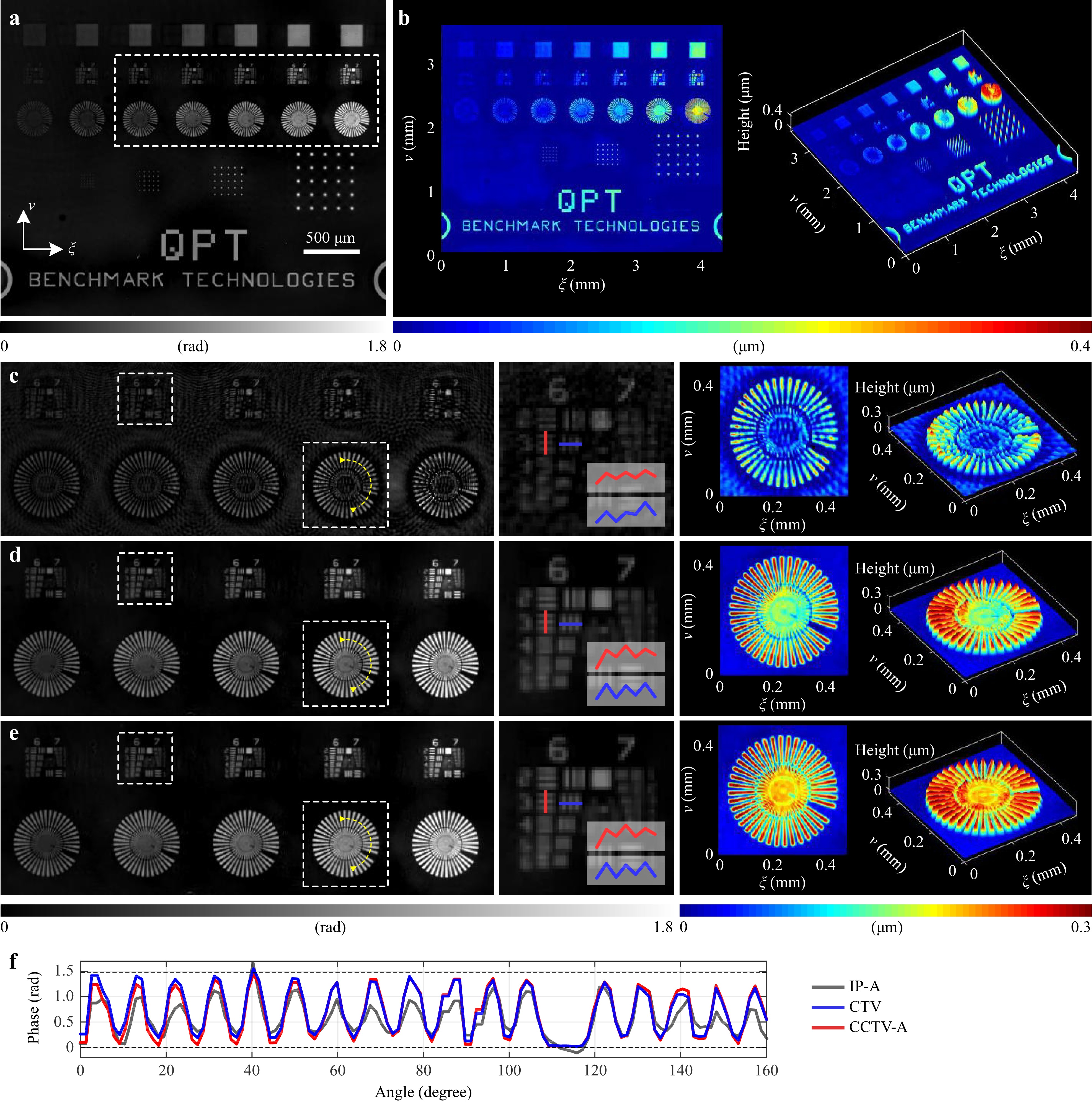
Fig. 4 Experimental comparison of different phase retrieval algorithms with a quantitative phase resolution target. a Full field-of-view phase reconstruction by the proposed CCTV-A method. b The calculated surface profile corresponding to a. c, d and e show the retrieved phase and height profiles by the IP-A, CTV, and CCTV-A methods, respectively. f The cross-sectional phase profiles, where the dashed line indicates the calculated theoretical phase value.
Similar improvements in the CCTV method over the IP and CTV methods were also observed in the imaging results of an amplitude object. Fig. 5 compares the amplitudes of a positive 1951 USAF test target (Thorlabs, Inc.) retrieved by the IP-A, CTV, and CCTV-A methods. Quantitatively, the RMSEs of the retrieved amplitude profiles 1/2 in Fig. 5d are 0.331/0.338, 0.240/0.239, 0.238/0.232 for the IP-A, CTV and CCTV-A methods, respectively. Furthermore, as indicated by a qualitative visual comparison, the IP method suffers from high reconstruction noise, and the CCTV model improves the performance of CTV by suppressing artifacts with no loss of spatial resolution.
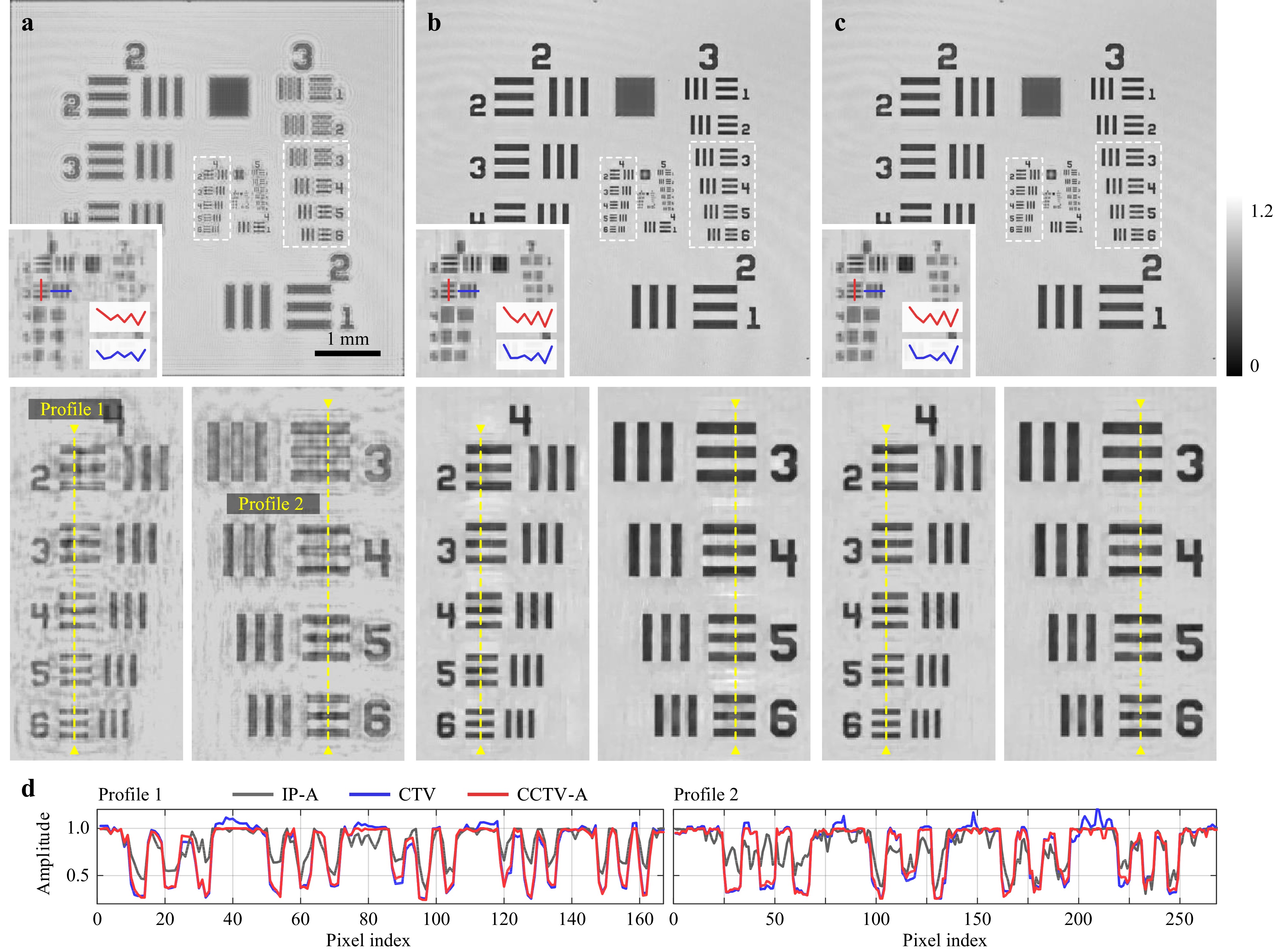
Fig. 5 Experimental comparison of different phase retrieval algorithms with an amplitude resolution target. a, b and c show the retrieved amplitude using the IP-A, CTV, and CCTV-A algorithms, respectively. The inset indicates the finest structures resolved by the corresponding method. Below are the corresponding enlarged areas. d Cross-sectional profiles.
-
In the regularized inverse problem of Eq. 3, the fidelity function
$ F({\boldsymbol{x}}) $ is a (almost everywhere) differentiable function whereas the regularizer$ R({\boldsymbol{x}}) $ is a non-differentiable function. Because we are dealing with real-valued functions over complex-valued variables, CR-calculus is adopted127. The gradient of$ F({\boldsymbol{x}}) $ is given by112$$ \nabla_{{\boldsymbol{x}}} F({\boldsymbol{x}}) = \frac{1}{2} {\boldsymbol{A}}^\mathsf{H} {\rm{diag}} \left( \frac{{\boldsymbol{Ax}}}{|{\boldsymbol{Ax}}|} \right) \left( |{\boldsymbol{Ax}}| - {\boldsymbol{y}} \right) $$ (5) where
$ (\cdot)^\mathsf{H} $ denote the conjugate transpose (Hermitian) operator. Non-smoothness only occurs when$ {\boldsymbol{Ax}} $ has zero entries, which, as we will show below, does not affect the algorithm’s convergence behavior.The difficulty in minimizing the objective function mainly arises from the non-differentiability of
$ R({\boldsymbol{x}}) $ . The proximal gradient method provides a general framework for solving composite non-smooth optimization problems in the form of Eq. 3 by minimizing the non-differentiable$ R({\boldsymbol{x}}) $ via its proximal operator$ {\rm{prox}}_{\gamma R} $ , which is defined as128$$ {\rm{prox}}_{\gamma R}({\boldsymbol{v}}) = \mathop{{\rm{argmin}}}\limits_{{\boldsymbol{x}}} R({\boldsymbol{x}}) + \frac{1}{2\gamma} \| {\boldsymbol{x}} - {\boldsymbol{v}} \|_2^2 $$ (6) where
$ \gamma > 0 $ is the step size. Notice that Eq. 6 coincides with an image denoising problem, with$ R({\boldsymbol{x}}) $ serving as a regularization function. For the CCTV regularizer, the denoising subproblem can be solved efficiently using the gradient projection algorithm introduced in the next subsection. The proximal gradient algorithm proceeds by iteratively applying a gradient update and proximal update. A variant using the Nesterov’s acceleration technique was adopted129, as shown in Algorithm 1. The accelerated proximal gradient (APG) algorithm is also known as the fast iterative shrinkage thresholding algorithm (FISTA)130. APG is well known for its superior convergence speed over the basic proximal gradient algorithm in the convex setting. Through numerical studies, we empirically demonstrate that it also helps to speed up convergence for the nonconvex phase retrieval problem.Algorithm 1 Accelerated proximal gradient algorithm Input: Initial guess $ {\boldsymbol{x}}^{(0)} $ , step size$ \gamma $ ,$ \beta_t = t/(t+3) $ , and iteration number$ T $ .1: $ {\boldsymbol{u}}^{(0)} = {\boldsymbol{x}}^{(0)} $ 2: for $ t = 1,2,\dots,T $ do3: $ {\boldsymbol{v}}^{(t)} = {\boldsymbol{u}}^{(t-1)} - \gamma \nabla_{{\boldsymbol{u}}} F({\boldsymbol{u}}^{(t-1)})\;\; $ $\triangleright $ Gradient update4: $ {\boldsymbol{x}}^{(t)} = {\rm{prox}}_{\gamma R}({\boldsymbol{v}}^{(t)})\;\; $ $\triangleright $ Proximal update via Alg. 25: $ {\boldsymbol{u}}^{(t)} = {\boldsymbol{x}}^{(t)} + \beta_t({\boldsymbol{x}}^{(t)} - {\boldsymbol{x}}^{(t-1)}) $ 6: end for -
The proximal update step in Eq. 6 involves solving a CCTV-regularized image denoising subproblem. It is a convex optimization problem when
$ C $ is closed and convex. No exact closed-form solution to this problem is available. Thus, an iterative solver should be invoked at every iteration. We followed the approach proposed in Refs. 95,131 and consider solving the primal problem via its dual, which is given by$$ \mathop{{\rm{min}}}\limits_{{\boldsymbol{w}} \in S} \, \left\{ G({\boldsymbol{w}}) \equiv - \| {{\cal H}}_C({\boldsymbol{v}} - \gamma {\boldsymbol{D}}^\mathsf{H} {\boldsymbol{w}}) \|_2^2 + \| {\boldsymbol{v}} - \gamma {\boldsymbol{D}}^\mathsf{H} {\boldsymbol{w}} \|_2^2 \right\} $$ (7) where
$ {\boldsymbol{w}}\in \mathbb{C}^{2n} $ denotes the dual variable,$ {\cal{H}}_C({\boldsymbol{x}}) \stackrel{\text{def}}{=} {\boldsymbol{x}} - {\cal{P}}_C({\boldsymbol{x}}) $ with$ {\cal{P}}_C $ representing the Euclidean projection operator on$ C $ , and$ S $ denotes the convex set which contains all$ {\boldsymbol{w}}\in \mathbb{C}^{2n} $ that satisfy$$ \| {\boldsymbol{w}} \|_\infty \leq \lambda $$ (8) where
$ \| {\boldsymbol{w}} \|_\infty = \max_i |w_i| $ . As shown in the Supplementary Document, the desired primal optimal solution$ {\boldsymbol{x}}^\star $ is related to the dual optimal solution$ {\boldsymbol{w}}^\star $ through the following equation:$$ {\boldsymbol{x}}^\star = {\cal{P}}_C ({\boldsymbol{v}} - \gamma {\boldsymbol{D}}^\mathsf{H} {\boldsymbol{w}}^\star) $$ (9) The problem of Eq. 7 can be effectively solved using the gradient projection algorithm, where the dual variable is iteratively updated by a gradient step followed by a projection operation
$ {\cal{P}}_S(\cdot) $ onto the set$ S $ . An accelerated variant of the algorithm is presented in Algorithm 2. The Wirtinger gradient of the dual objective function$ G({\boldsymbol{w}}) $ is given by131$$ \nabla_{{\boldsymbol{w}}} G({\boldsymbol{w}}) = -\gamma {\boldsymbol{D}} {\cal{P}}_C ( {\boldsymbol{v}} - \gamma {\boldsymbol{D}}^\mathsf{H} {\boldsymbol{w}} ) $$ (10) Algorithm 2 Accelerated gradient projection algorithm Input: Observation $ {\boldsymbol{v}} $ , parameter$ \gamma $ , step size$ \eta $ ,$ \beta_t = t/(t+3) $ , and subiteration number$ T_{{\rm{sub}}} $ .1: $ {\boldsymbol{w}}^{(0)} ={\bf{0}} $ ,$ {\boldsymbol{z}}^{(0)} = {\boldsymbol{w}}^{(0)} $ 2: for $ t = 1,2,\dots,T_{\rm{sub}} $ do3: $ {\boldsymbol{w}}^{(t)} = {\cal{P}}_S \left( {\boldsymbol{z}}^{(t-1)} - \eta \nabla_{{\boldsymbol{z}}} G( {\boldsymbol{z}}^{(t-1)} ) \right) $ 4: $ {\boldsymbol{z}}^{(t)} = {\boldsymbol{w}}^{(t)} + \beta_t ({\boldsymbol{w}}^{(t)} - {\boldsymbol{w}}^{(t-1)}) $ 5: end for 6: $ {\boldsymbol{x}} = {\cal{P}}_C({\boldsymbol{v}} - \gamma {\boldsymbol{D}}^\mathsf{H}{\boldsymbol{w}}^{(T_{\rm{sub}})}) $ -
In the above subsections, we introduce the proximal gradient algorithm and the corresponding denoising algorithm for the proximal update. We now show that the algorithm parameters, namely the step sizes
$ \gamma $ and$ \eta $ , can be predetermined based on the measurement scheme and the sparsifying transform.Considering the nonconvexity of the problem of Eq. 3, we present a weaker result by showing the convergence of the basic (non-accelerated) proximal gradient algorithm, which is summarized by the following theorem. The detailed proof is provided in the Supplementary Document. Furthermore, extensive numerical studies have demonstrated that the accelerated algorithm converges following the same step size selection rule.
Theorem 1 The basic proximal gradient algorithm (with
$ \beta_t \equiv 0 $ in Algorithm 1) for the problem of Eq. 3 converges to a stationary point using a fixed step size$ \gamma $ that satisfies$$ \gamma \leq \frac{2}{\rho({\boldsymbol{A}}^\mathsf{H}{\boldsymbol{A}})} $$ (11) where
$ \rho(\cdot) $ denotes the spectral radius.The above theorem is an extension of the gradient descent algorithm132 to the more general class of the proximal gradient algorithms.
The sampling matrix
$ {\boldsymbol{A}} $ depends only on the physical model. Thus, the step size can be known a priori. Recall that the sampling matrix comprises a circular convolution operator$ {\boldsymbol{Q}} $ and an image cropping operator$ {\boldsymbol{C}} $ . Circular convolution can be efficiently calculated via FFTs as$ {\boldsymbol{Q}} = {\boldsymbol{F}}^{-1}{\rm{diag}}({\boldsymbol{h}}){\boldsymbol{F}} $ , where$ {\boldsymbol{F}} $ is the Fourier matrix and$ {\boldsymbol{h}} $ is the transfer function. Note that$ |{\boldsymbol{h}}|={\bf{1}} $ . Thus,$ {\boldsymbol{Q}} $ is a unitary matrix that satisfies$ {\boldsymbol{Q}}^\mathsf{H}{\boldsymbol{Q}} = {\boldsymbol{I}} $ , where$ {\boldsymbol{I}} $ is the identity matrix. It can be easily verified that$ \rho({\boldsymbol{A}}^\mathsf{H}{\boldsymbol{A}}) \leq 1 $ , which, according to Theorem 1, implies that we should use step size$ \gamma = 2 $ for the proximal gradient algorithm. This choice of step size is in fact nontrivial and generally applicable to any passive measurement scheme.The next theorem establishes the convergence of the accelerated gradient projection algorithm to solve the convex denoising subproblem via its dual (Eq. 7). The proof can be found in the Supplementary Document.
Theorem 2 Assuming that the constraint set
$ C $ is closed and convex, the accelerated gradient projection algorithm for the problem of Eq. 7 converges to the global optimum using a fixed step size$ \eta $ that satisfies$$ \eta \leq \frac{1}{\gamma^2 \rho({\boldsymbol{D}}^\mathsf{H}{\boldsymbol{D}})} $$ (12) Theorem 2 suggests that the step size for the denoising algorithm can also be determined beforehand based on
$ \gamma $ given by Theorem 1 and the sparsifying transform$ {\boldsymbol{D}} $ . Specifically, for the finite-difference operator, we show in the Supplementary Document that$ \rho({\boldsymbol{D}}^\mathsf{H}{\boldsymbol{D}}) \leq 8 $ , which, together with$ \gamma = 2 $ , suggests$ \eta = 1/32 $ for this particular case. The convergence established by Theorem 1 assumes that an exact solution to the denoising subproblem is obtained at each iteration. The algorithm may converge to a suboptimal solution when the proximal update is inexact, as with the CCTV regularizer. Readers can refer to Ref. 133 and references therein for convergence results regarding inexact proximal gradient algorithms. Therefore, the iteration number used for the gradient projection algorithm should be chosen as a balance between reconstruction quality and computation efficiency. -
We performed numerical studies based on the same in-line holographic imaging model as described in the experiment section to quantitatively evaluate the algorithmic behaviors and further shed light on our empirical observations and theoretical results. The wavelength was set to 500 nm, the pixel size was 5 µm, and the imaging distance was 5 mm. Eight standard test images of size 256×256 were used to generate the virtual phase objects for the simulation. The phase of the object was assumed to have a range of
$ [0,\pi] $ . The objects have a uniform amplitude distribution and were zero-padded to avoid boundary artifacts. Additive white Gaussian noise was added to each hologram such that the signal-to-noise ratio (SNR) was 20 dB by default. We calculated the phase RMSE as a metric to quantitatively compare the reconstruction quality of different methods.In all numerical studies, the algorithms were initialized with an initial estimate of
$ {\boldsymbol{x}}^{(0)} = {\boldsymbol{A}}^\mathsf{H} {\boldsymbol{y}} $ . The algorithms were implemented using MATLAB on a personal computer with Core i7-11700F CPU @ 2.50GHz (Intel) and 16 GB of RAM. The MATLAB code is publicly available in Ref. 134. -
We first investigated the influence of the subiteration number
$ T_{\rm{sub}} $ of the gradient projection denoising algorithm on the convergence of the proximal gradient algorithm. As previously pointed out,$ T_{\rm{sub}} $ is a key hyperparameter that should be determined beforehand. We ran the APG algorithm for 1000 iterations using different$ T_{\rm{sub}} $ values ranging from one to ten. Meanwhile, four regularization parameters,$ \lambda = 1\times 10^{-3} $ ,$ 3\times 10^{-3} $ ,$ 1\times 10^{-2} $ , and$ 3\times 10^{-2} $ were considered for comparison. To quantify the convergence behavior of the inexact APG algorithms, we calculated the relative error of the final objective function value for each$ T_{\rm{sub}} $ relative to that with$ T_{\rm{sub}} = 10 $ . Fig. 6a indicates that the relative error decreases monotonically as$ T_{\rm{sub}} $ increases, and thus, a more accurate proximal update can be obtained by increasing the number of subiterations. We empirically selected the smallest$ T_{\rm{sub}} $ that yielded an error below$ 1\% $ as the optimal choice. Another observation made from Fig. 6a is the dependence of$ T_{\rm{sub}} $ on regularization parameter$ \lambda $ . As$ \lambda $ increases, one needs more subiterations for the denoising algorithm to obtain an adequate solution. This seems quite natural, considering the nonlinear nature of the denoising operation. A larger$ \lambda $ imposes a stronger regularization force on the image, thus requiring more linear iterative steps to approximate the solution.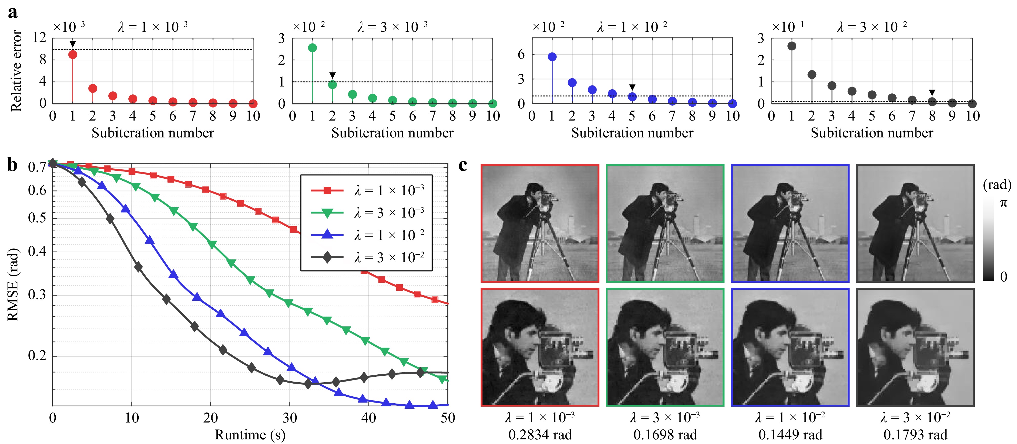
Fig. 6 Comparison of different hyperparameter selections based on simulations. a Relative error against subiteration number
$ T_{\rm{sub}} $ for different regularization parameters$ \lambda $ . The dashed lines indicate the value of 1%, and the downward-pointing triangles indicate the optimal choice of subiteration number that satisfies the error criterion. b Root-mean-square error against runtime for different$ \lambda $ when using the corresponding optimal$ T_{\rm{sub}} $ in a. c Phase obtained by running the algorithms for 50 s. The second row shows the enlarged areas. The regularization parameters and RMSEs are shown below. No physical constraints are considered in this simulation.Another hyperparameter of great importance is the regularization parameter
$ \lambda $ , which offers a tradeoff between model consistency and signal priors. We compared different selections of$ \lambda $ in terms of both the reconstruction quality and computational efficiency. Fig. 6b plots the convergence curves against runtime, where the optimal$ T_{\rm{sub}} $ was used for each$ \lambda $ , that is,$ T_{\rm{sub}} = 1 $ for$ \lambda = 1\times 10^{-3} $ ,$ T_{\rm{sub}} = 2 $ for$ \lambda = 3\times 10^{-3} $ ,$ T_{\rm{sub}} = 5 $ for$ \lambda = 1\times 10^{-2} $ , and$ T_{\rm{sub}} = 8 $ for$ \lambda = 3\times 10^{-2} $ . A larger regularization parameter can help accelerate the convergence at the beginning stage. However, the final result tends to be over-smoothed, as shown in Fig. 6c. Therefore, we set$ \lambda = 1\times 10^{-2} $ for balanced performance in terms of speed and accuracy. -
Having determined the optimal hyperparameters for the complex TV, we evaluated the effect of incorporating additional physical constraints. Fig. 7 shows the results obtained using no constraints, support constraint, absorption constraint, or both. For the support constraint, the support region was set to the central
$ 256\times 256 $ pixels of the image. The introduction of the absorption constraint can significantly improve the overall quality, while the support constraint can help suppress artifacts at the boundaries. Incorporating physical constraints also helps accelerate convergence.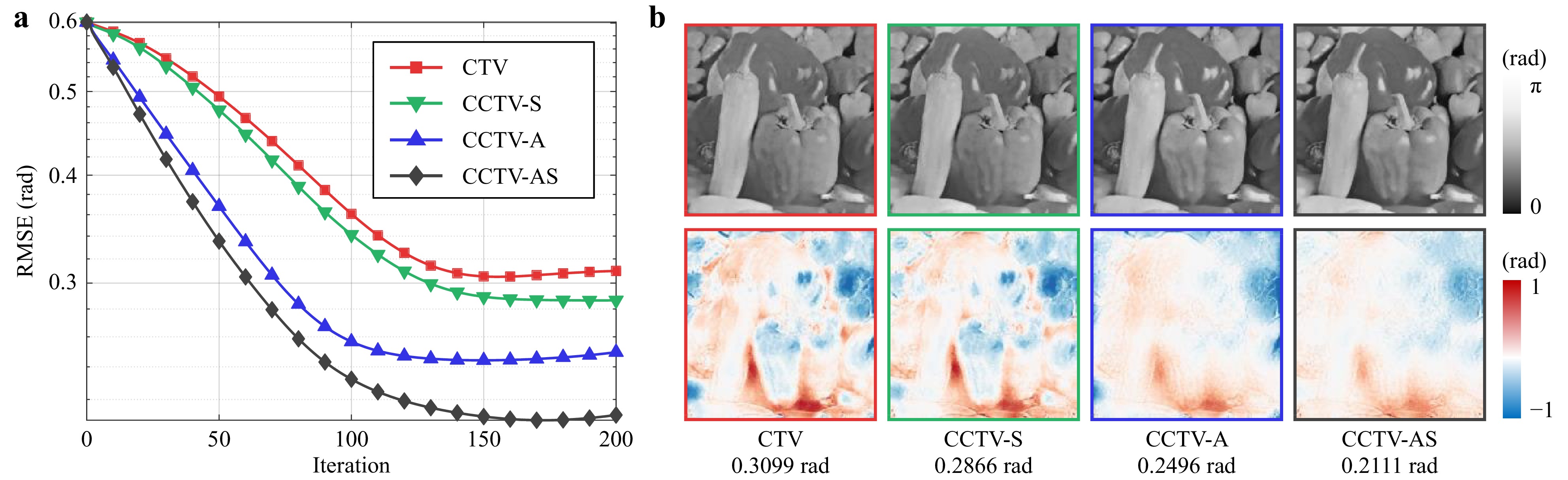
Fig. 7 Comparison of convergence speed and reconstruction quality with different physical constraints. a The RMSE is plotted against the iteration number. b The upper and lower rows show the reconstructed phase after 200 iterations and the corresponding phase residuals, respectively. The calculated phase RMSEs are shown below.
-
The inherent ill-posedness of single-shot phase retrieval leads to high sensitivity to measurement noise. To quantitatively compare the phase reconstruction quality under noisy conditions, we added different levels of additive white Gaussian noise with an SNR ranging from 5 to 30 dB to the simulated hologram, as shown in Fig. 8a. The corresponding phases retrieved by the CCTV-AS method are presented in Fig. 8c. The CCTV method can achieve high-quality phase retrieval under moderate-noise conditions. However, when the hologram is severely degraded by measurement noise, a larger regularization parameter
$ \lambda $ is required to suppress reconstruction artifacts. The retrieved phase may then exhibit a staircase artifact when the regularization parameter is too large, which is an inherent problem for TV-based regularizers. Therefore, more advanced image priors are required to achieve better reconstruction quality under noisy conditions.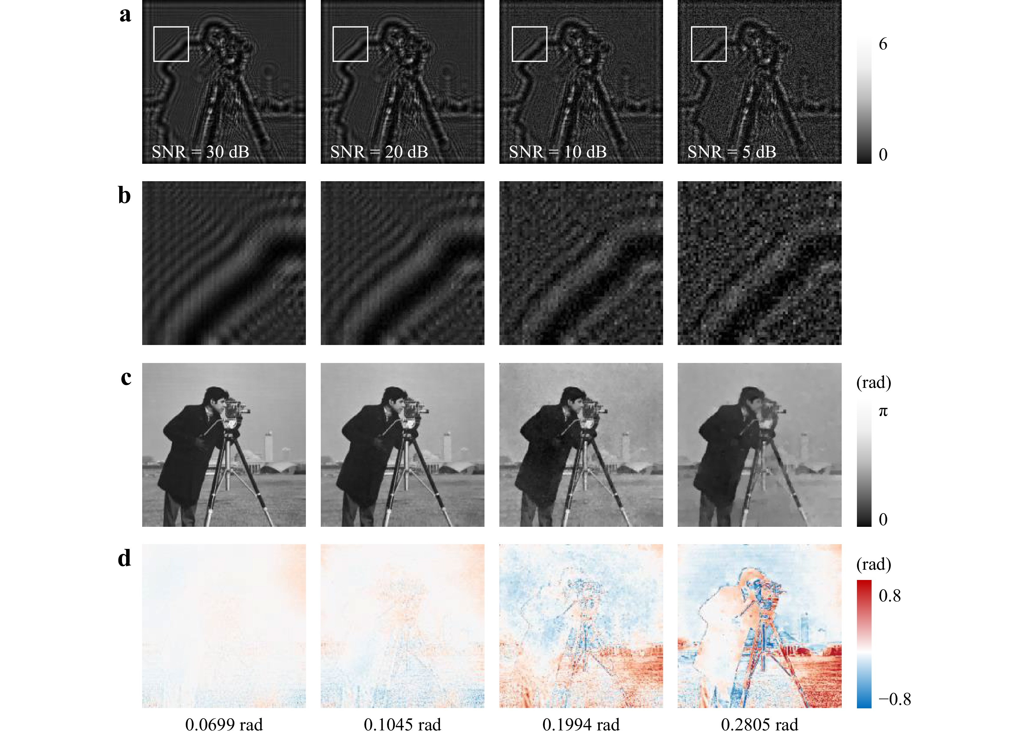
Fig. 8 Effect of measurement noise on reconstruction quality. a Simulated noisy holograms with different SNRs. b Corresponding enlarged areas of a. c Retrieved phase by the CCTV-AS method. d Phase residuals of c. The calculated phase RMSEs are shown below.
-
To further examine the generalizability of the CCTV model, we tested the algorithm on various test images and compared it with IP and CTV methods. The results are shown in Fig. 9. The conventional IP algorithm generally suffers from a high reconstruction error because the physical constraints alone are insufficient to suppress the twin-image artifact. On the other hand, the CTV model often yields visually appealing results, yet its performance is highly dependent on the sparsity of the scene. For example, the CTV model tends to perform well for scenes with very sparse gradients, such as the House image, but it may be unsuitable for retrieving complex scenes, such as the Goldhill and Mandrill images. In all cases, the CCTV model offers the best reconstruction quality owing to the combination of sparsity priors and physical constraints. We also set
$ \lambda = 1\times 10^{-2} $ as fixed throughout the simulation experiments. This implies that the selection of$ \lambda $ is not very sensitive to the scene content.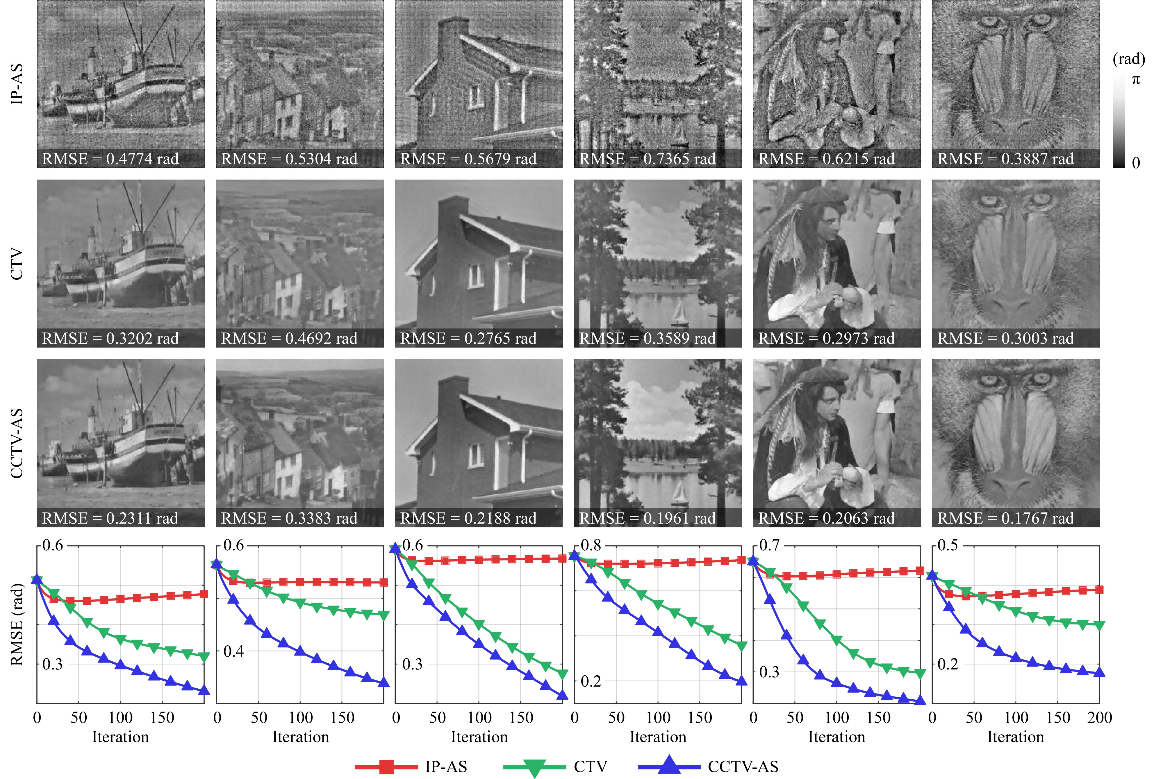
Fig. 9 Comparison of the IP-AS, CTV, and CCTV-AS methods for various test images (from left to right: Ship, Goldhill, House, Lake, Male, Mandrill). The upper three rows show the reconstructed phase by the three methods. The bottom row plots the RMSE against the iteration number.
-
We also empirically validated the effectiveness of Nesterov’s method for the nonconvex phase retrieval problem by comparing the APG algorithm with the non-accelerated version in both unconstrained and constrained cases, as shown in Fig. 10a, b, respectively. Nesterov’s method significantly improved the convergence speed in both cases. The APG algorithm involves only an additional extrapolation step per iteration, whose time consumption is negligible compared with the gradient and proximal update steps. The empirical success of Nesterov’s method can be explained partly by the similarity between the amplitude-based fidelity function and the convex least-squares formulation107.
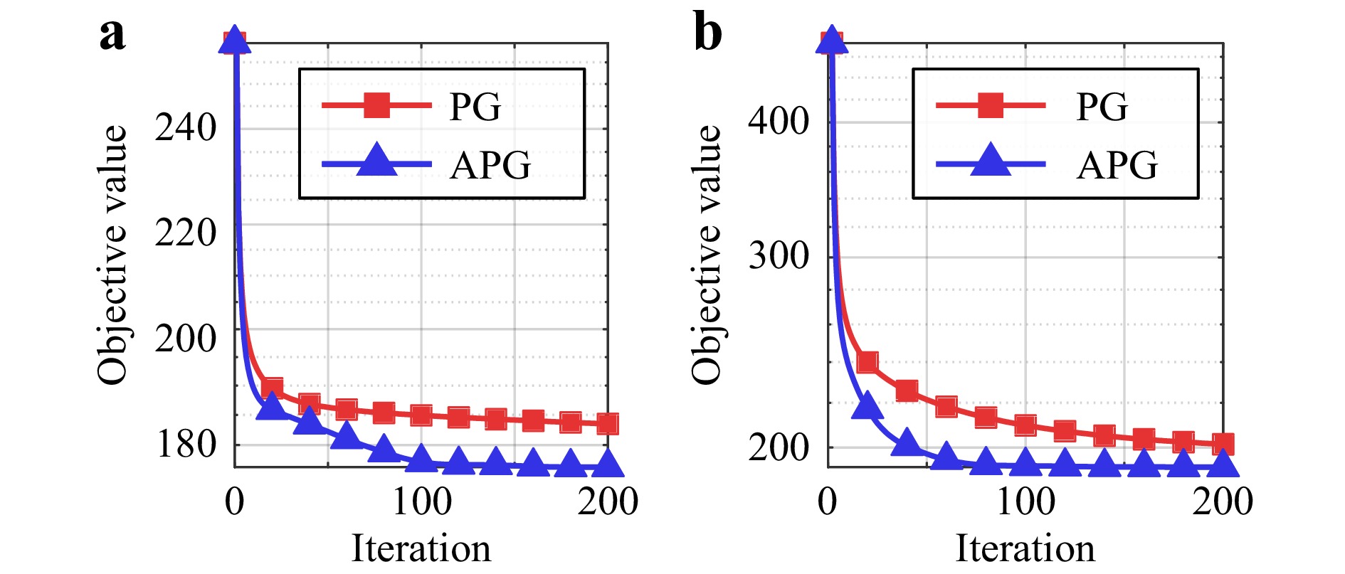
Fig. 10 Convergence of the proximal gradient (PG) algorithm and its accelerated variant (APG) in a unconstrained case and b constrained case.
-
We have proposed a unified compressive phase retrieval framework for in-line holography that combines the complex total variation and physical knowledge of the wavefield. The resulting CCTV model can characterize the sparse nature of complex real-world scenes while leveraging physically tractable constraints to further improve imaging quality, as confirmed by both simulated and optical experiments. In addition, we conducted a detailed theoretical analysis from a mathematical viewpoint, which provides general guidance for algorithm parameter selection to ensure convergence, obviating the need for laborious manual tuning. We emphasize that the proposed framework is generally applicable to various optical configurations and can easily adapt to other physical constraints and sparsifying operators.
Although numerically extending the proposed algorithmic framework to coherent diffraction imaging is straightforward, retrieving complex-valued images from a single far-field diffraction pattern remains challenging. Future work will explore more advanced image priors that enable snapshot coherent diffraction imaging of complex samples135. Another direction for future research is to achieve quantitative phase imaging of objects with a large phase shift, as only weak phase objects have been tested in this work. Comparison of the proposed method with other existing quantitative phase imaging methods also remains to be studied in the future136,137.
-
The authors acknowledge the National Natural Science Foundation of China (Grant No. 61827825) for financial support. The authors would also like to thank the anonymous reviewers for their constructive comments and suggestions, which improved the presentation of the paper. Part of this paper was posted as a preprint138 before submission.


 DownLoad: