Investigating a corrective online measurement method for the tool influence function in millimetre spot-sized ion beam figuring

New-generation synchrotron radiation and X-ray free-electron laser facilities produce ultra-brilliant, highly coherent X-ray beams, offering a unique approach to explore the nanostructure and fundamental processes of matter¹. Among the most prevalent optical components are X-ray mirrors, which collimate, focus, and deflect X-ray beamlines. Importantly, X-ray^2–6 mirrors are crucial ultra-precision optical components; the short wavelength of X-rays necessitates the reflection of photons only at the grazing angle of incidence on an extremely high-precision and smooth surface. Consequently, there are stringent requirements to limit surface irregularity on all spatial scales. Among them, low-frequency form errors are typically defined as form components with spatial wavelengths ranging from 1 mm to the full aperture of the optical component. These errors introduce aberrations into the optical system, resulting in distorted and deformed imaging⁷. To enhance the imaging quality, the accuracy in this low-frequency band must be below 1 nm. However, form errors with spatial wavelengths ranging from 10 to 1 mm approach the mid-frequency range, necessitating the use of more precise figuring tools and processes.

There are two approaches to overcome form errors within the aforementioned range. One approach is to use a larger tool to cover the form errors, which are eliminated based on the smoothing effect⁸. However, it is hard to maintain the lower-frequency form errors, which may require the introduction of an additional figuring process. The other approach is to use a small tool to figure the form errors point-wise, by controlling the tool influence function (TIF) such that it traverses the entire surface with varying dwell times or velocities^9,10. This approach is more accurate, but requires the TIF to be sufficiently small and stable. To fully cover the form errors within this range, the full width at half maximum (FWHM) of the TIF should be reduced to approximately 0.5 mm¹¹. However, typical processing technologies such as magnetorheological finishing (MRF) encounter challenges in reducing the TIF size to meet specific requirements; furthermore, there are other limitations. For example, during MRF processing, the removal efficiency fluctuates with the polishing particle consumption, and a D-shaped TIF reduces the convergence efficiency of form errors and introduces tool mark errors^12–15. Compared with the aforementioned methods, ion beam figuring (IBF)^16–18 is a non-contact processing technology with high determinism and accuracy. IBF removes the material at the atom level by physical sputtering. Its distinctive advantage lies in its rotationally symmetric Gaussian TIF. By using various sizes of ion diaphragms and grids, the FWHM of the TIF can be easily reduced from tens of millimetres to even 0.5 mm, enabling both coarse and fine error correction^19–21. Canon’s research showed that a TIF with an FWHM of 0.5 mm could significantly reduce form errors near a spatial wavelength of 1 mm²². Above all, IBF with a small-sized TIF can effectively and deterministically figure form errors within this range; this process is referred to as millimetre spot-sized IBF in this paper. Typically, the FWHM of a small-sized TIF is below 2 mm.

Therefore, the precise measurement of the TIF is imperative, as it provides the material removal distribution per unit time. This information is subsequently used to calculate the dwell time, whose quality directly impacts the accuracy and convergence of IBF²³. To obtain this information, the TIF can be directly acquired by a static processing test, where the TIF dwells at the single point to generate the removal distribution^24,25. Nevertheless, the TIF can also be measured online more efficiently by establishing the relationship between the TIF and beam current density (BCD) distribution. This is achieved by the static processing test and by scanning the ion beam with the Faraday cup (FC). According to the Sigmund theory²⁶, it is considered that the TIF and BCD are consistent. In other words, the FWHM remains the same, while the peak BCD is linearly related to the peak removal rate (PRR). Hence, the TIF can be directly measured with the BCD distribution acquired by FC scanning. To illustrate this, Zhang et al.²⁷ approximated the TIF by using the measured BCD distribution, while Tang et al.²⁸ established a TIF measurement model based on FC measurement results for silicon and fused quartz materials, which was verified by experiments. Compared with the former, the online measurement method is preferred owing to its rapid implementation, which renders it advantageous for practical application.

Although the two aforementioned measurement methods can both be applied to small-sized TIFs with FWHMs less than 2 mm, the static processing test is generally the only method to precisely measure a small-sized TIF. In 2000, Seah et al. noted the existence of the convolution effect in FC scanning, which is closely related to the FC aperture. When the ion beam size approaches that of the FC aperture, the measurement becomes inaccurate^29,30. In this scenario, the online measurement results no longer accurately provide the TIF distribution. For example, as shown in Fig. 1, the real FWHM of the TIF is 0.51 mm, while the FWHM corresponding to the measured BCD distribution is 0.93 mm, indicating a wider distribution with a measurement error of 82.4%. The relationship between them is no longer simply linear; the shape distribution also changes. Previous studies primarily focused on large-sized TIFs; further, the measurement errors in the TIF were often attributed to measurement inaccuracies or the influence of the neutraliser²⁸. However, the experimental observations reveal that the discrepancies between the TIF and measured BCD distribution are more pronounced in small-sized TIFs and exceed explainable limits. Considering the discrepancy in the FWHM, Zhang et al.³¹ used a back-propagation neural network to model the nonlinear relationship between the FWHM of the TIF and measured the BCD distribution. However, their approach only described the discrepancy to a certain extent, without an in-depth analysis, thus failing to fundamentally address the issue. At present, the convolution effect in FC scanning has only been explained from the physics perspective, and the resulting inaccuracy of the existing online measurement method has not yet been clarified.

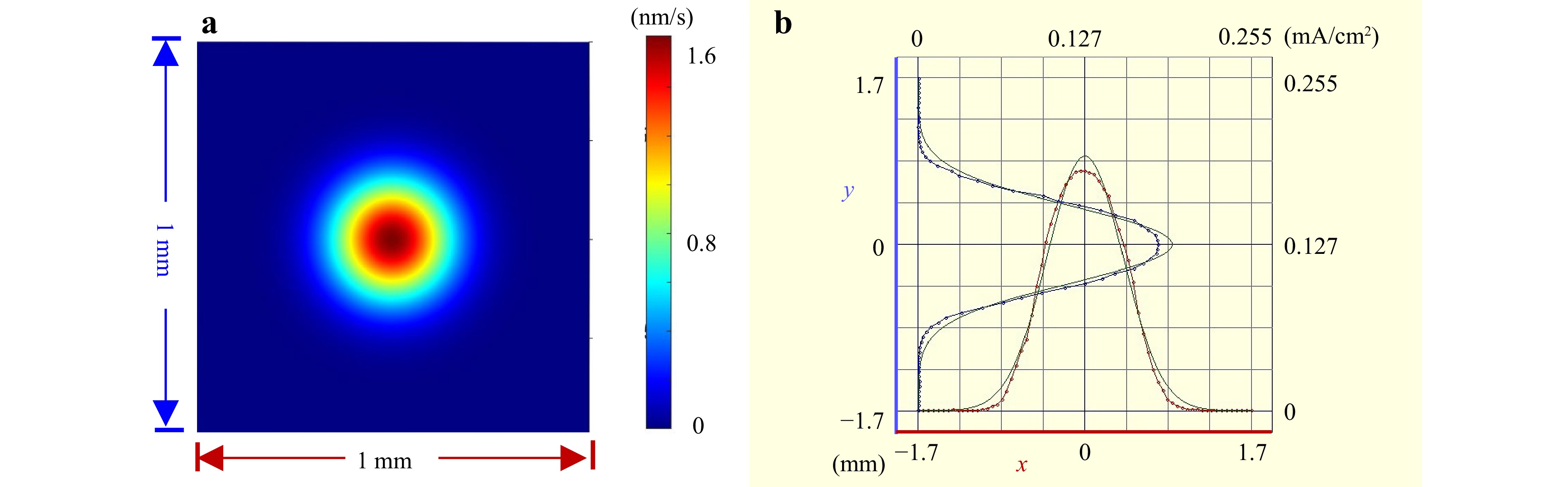
Fig. 1  Illustration of the measurement error for a small-sized TIF by a previous online method. a TIF with an FWHM of 0.51 mm acquired by the static processing test. b Corresponding measured BCD distribution with an FWHM of 0.93 mm along two directions. (The red and blue curves represent the original measurement data acquired from X and Y direction scans, respectively, while the green curves indicate the Gaussian fitting results for these data).

Above all, the development of high-precision online measurement for the small-sized TIF is urgent, because the application of small-sized TIF generally lasts for a long time, especially for large-aperture mirrors, making that the real-time monitoring, evaluation and compensation of TIF stability is essential. Thus far, this could not be achieved by the static processing test, with which the TIF could only be acquired offline and evaluated after completion of the experiment. The compensation of TIF changes can only be considered in the next figuring loop, not to mention the auxiliary time caused by the vacuum venting and pumping procedure in IBF. Given these requirements, the convolution effect in FC scanning needs to be incorporated into the online measurement method for small-sized TIFs, which is imperative to enhance the processing precision and efficiency with reliable feedback and process optimisation.

With the aforementioned aim, this study attempts to fill the research gap on the development of a high-precision online measurement method for small-sized TIFs in millimetre spot-sized IBF. This paper proposes an online measurement method for correcting the convolution effect. The proposed method not only allows for rapid measurements without the need for tedious experiments, but also improves the measurement accuracy for small-sized TIFs. The rest of the paper is organised as follows. The error analysis for the TIF measurement is provided in Section 2. In Section 3, a corrective online measurement method for the TIF is proposed. In Section 4, the convolution effect in the FC measurement is analysed by calculation. In Section 5, the accuracy of the method for small-sized TIFs is verified and the polishing experiment is conducted. The necessity of the method is discussed in Section 6. Finally, the work is summarised in Section 7.

Fig. 2 shows a flowchart of the IBF process integrated with the previously proposed online measurement method for the TIF, which is a critical input in dwell time optimisation. The existing TIF measurement method primarily involves coefficient calibration and TIF calculation. The former is generally performed once for each material. In this process, FC scanning and the static processing test are conducted to calibrate the critical proportional coefficient k between the BCD distribution and TIF. The FC is a conductive metal cup designed to collect charged particles^32–34. It features a small aperture at its front end to receive the ion beam, where the energy of the charged particles is absorbed and transformed into an electric current or electric current density^35,36. To fully acquire the BCD distribution, the aperture size of the FC is generally smaller than the diameter of the ion beam; hence, only a portion of the beam can pass through the aperture. During the scanning test, the ion beam moves along the X and Y axes to pass through the aperture. Considering that the ion beam emitted from the ion source undergoes shaping by the ion optical system, the BCD distribution $ {J_{{\text{real}}}}\left( {x,y} \right) $ has a perfect Gaussian shape, which can be represented by Eq. 1 as follows:

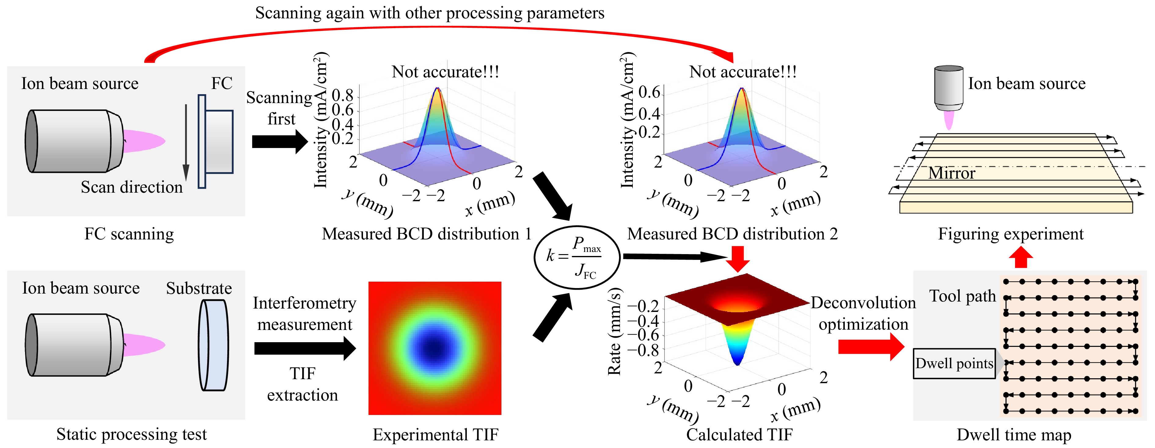
Fig. 2  Flowchart of the IBF process integrated with the previously proposed online measurement method for the TIF.

where $ \sigma $ represents the Gaussian distribution coefficient of the BCD distribution and $ {J_{\max }} $ is the real peak value of $ {J_{{\text{real}}}}\left( {x,y} \right) $. Correspondingly, the measured BCD distribution obtained by the FC can be represented by Eq. 2, which is expected to truly reflect the real BCD distribution.

where $ {J_{{\text{FC}}}} $ represents the measured peak BCD, which is considered to be equal to $ {J_{\max }} $.

According to the Sigmund theory^26,37, an ion beam with a Gaussian distribution can form a TIF with a Gaussian distribution on the optical surface, and the distribution of the real beam is consistent with the distribution of the TIF. Therefore, the corresponding TIF $ R\left( {x,y} \right) $ can be expressed by Eq. 3 as follows:

where $ {P_{\max }} $ represents the PRR of the TIF. For identical materials, the material removal rate at any point on the optical surface is influenced by the ion beam energy, spatial distribution, and incident angle. Under the conditions of a constant energy and angle, the sputtering yield remains stable; consequently, the quantity of material removed is theoretically proportional to the real BCD distribution. Therefore, after the completion of the static processing test, the measured TIF can be used to calibrate the proportional coefficient k, which is expressed as

Thus, given that the proportional coefficient k is calibrated for any material, the TIF can be calculated with the corresponding BCD distribution acquired by FC scanning, and is expressed as follows:

where $ FWH{M_{{\text{FC}}}} $ is the FWHM of the measured BCD distribution.

In the aforementioned TIF measurement procedure, it is assumed that the FC scanning perfectly acquires the BCD distribution emitted from the ion beam source, i.e., the measured BCD distribution is the same as the real BCD distribution. However, the presence of the convolution effect makes this difficult to achieve^29,38, as it is related to the size of the FC aperture and the measured BCD distribution. In millimetre spot-sized IBF, a small-sized TIF indicates a small-sized BCD distribution, rendering the convolution effect non-negligible. Once the BCD information is captured, the detected current value reflects the accumulated current within the aperture area, yielding an average rather than an instantaneous current density at a specific point. Therefore, as the ion beam diameter decreases, the existing convolution effect is amplified, leading to greater inaccuracy.

To better understand this, Fig. 3 provides an illustration of the measurement error for BCD distributions of different sizes. For larger-diameter ion beams, the BCD gradient variations are very small within a confined aperture range. Therefore, the average BCD is closer to the instantaneous value within the FC aperture. This indicates that the FC scanning is more accurate, making the TIF measurement more reliable. In this scenario, the calculated TIF is almost the same as that obtained from the static processing test. However, as the ion beam diameter decreases, the amplified convolution effect generates a considerable discrepancy between the measured and real BCD distributions owing to the larger local gradient of the BCD distribution. Therefore, the smaller the beam diameter, the greater the influence when the aperture size is unchanged. Consequently, the FWHM of the TIF markedly deviates from the measured BCD distribution, as shown in Fig. 1.

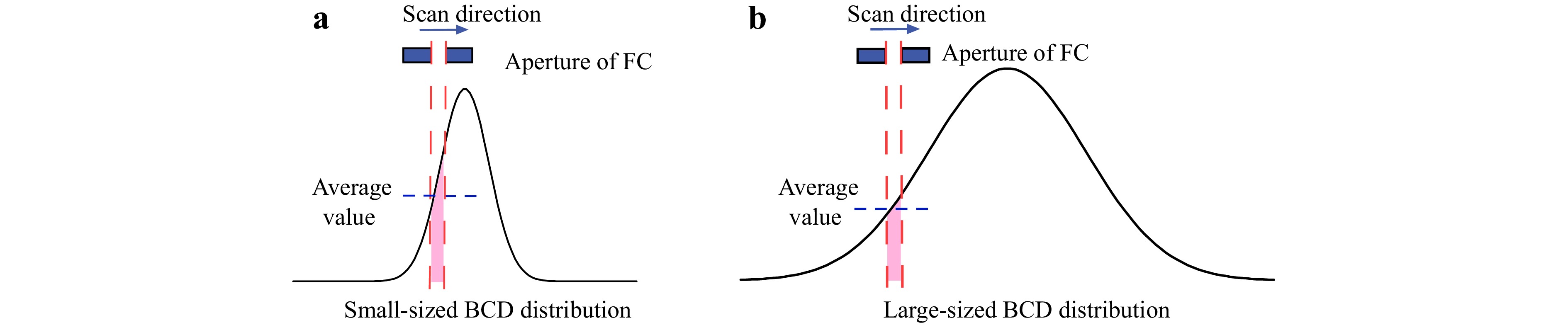
Fig. 3  Illustration of the measurement error for BCD distributions of different sizes. a Small-sized BCD distribution. b Large-sized BCD distribution.

To confirm the inapplicability of the previous measurement method for small-sized TIFs, a series of FC scanning and static processing tests were conducted (Fig. 4). The diameter of the grid was set to 10 mm, and the size of the ion beam was adjusted by varying the ion diaphragms and working distance. In these experiments, the dwell time for each static processing test was specifically set to ensure that its product with the measured peak BCD remained the same. If the previous TIF measurement method were to be applicable, then consistent product values should yield consistent removal depths for each test. The detailed experimental parameters are listed in Table 1. The ion source parameters remained constant and were stringently tested, ensuring maximum stability of the ion beam source. Thirty measurements were conducted at each sampling location and averaged to mitigate the high-frequency noise during scanning. Further, each test was conducted three times under different conditions, with the results averaged to ensure reliability.

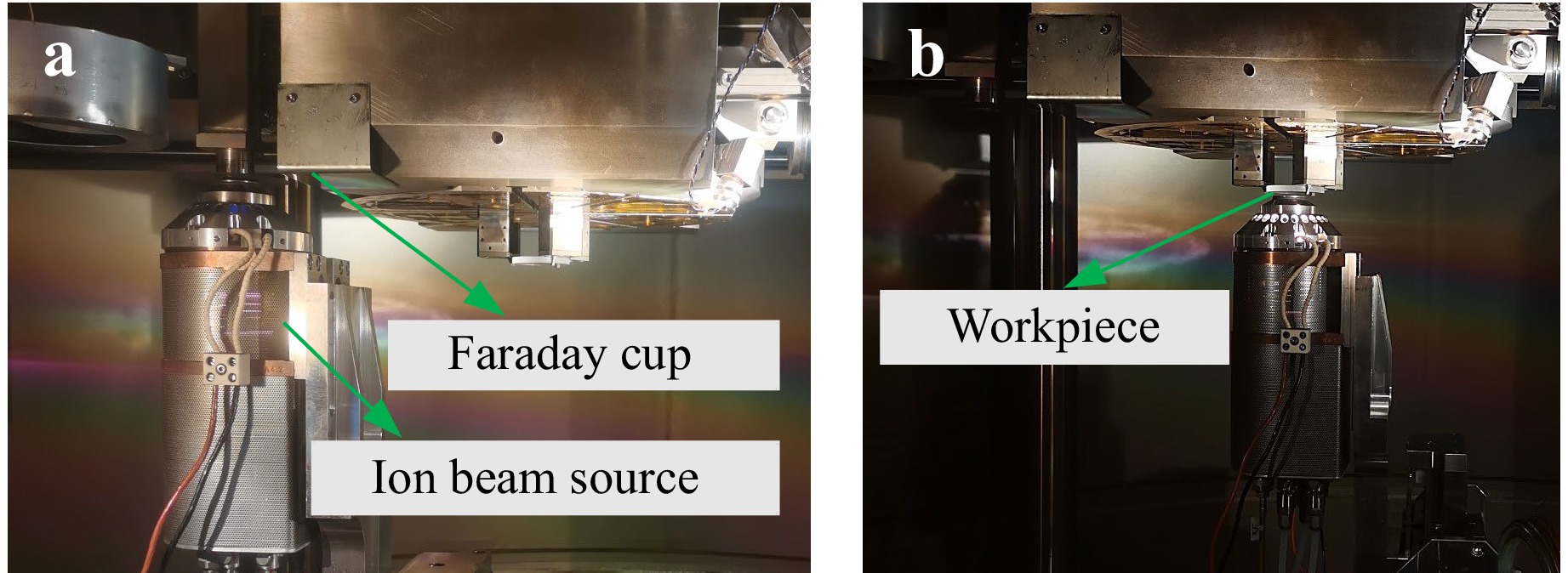
Fig. 4  Schematic of the experimental process. a FC scanning. b Static processing test.

The experimental results are shown in Fig. 5. When the FWHM of the TIF is sufficiently large, the removal depth is almost unchanged, indicating that the convolution effect can be ignored. As the FWHM of the TIF decreases below 2 mm, the removal depth increases exponentially, implying that the amplitude of the measured BCD distribution is increasingly underestimated. This indicates that a nonlinear relationship emerges between the TIF and the measured BCD distribution when the ion beam size is below a threshold, providing direct evidence of the non-negligible measurement error caused by the convolution effect for small-sized TIFs. This finding contradicts the Sigmund theory, and highlights the necessity of correcting the convolution effect for the high-precision measurement of small-sized TIFs.

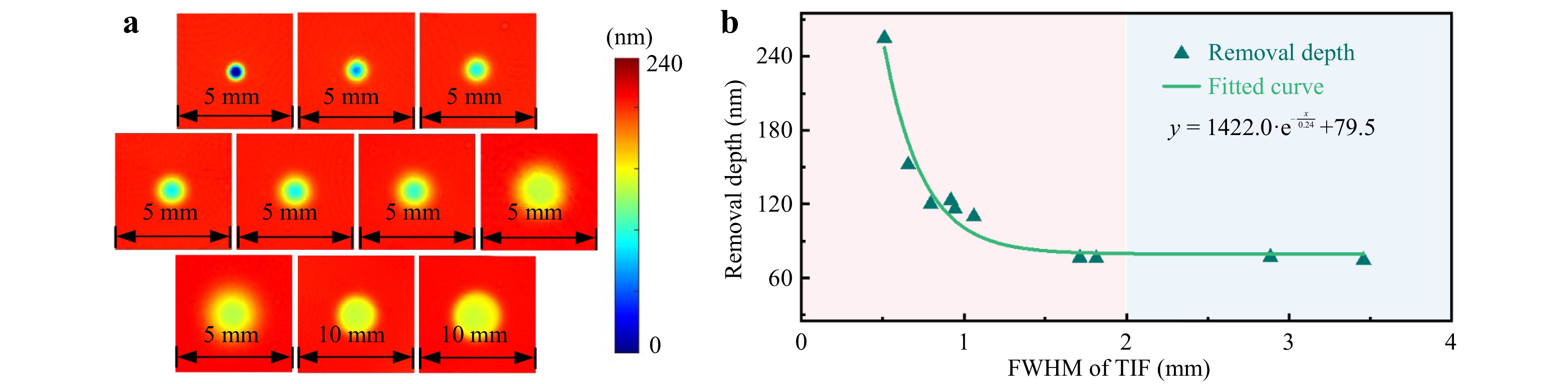
Fig. 5  Experimental results. a Measured removal distributions. b Relationship between the removal depth and FWHM of TIFs.

To enhance the accuracy of the TIF measurement, the correction for the convolution effect must be incorporated in the corrective online measurement method; this represents the most significant distinction of the proposed method from the previous method. The flowchart of the corrective measurement method is shown in Fig. 6, and comprises three stages. Compared with the previous method, an additional step of establishing the mapping relationship between the real and measured BCD distributions is introduced. Based on previous studies^29,30, the convolution effect during FC scanning can be mathematically explained by Eqs. 7, 8 as follows:

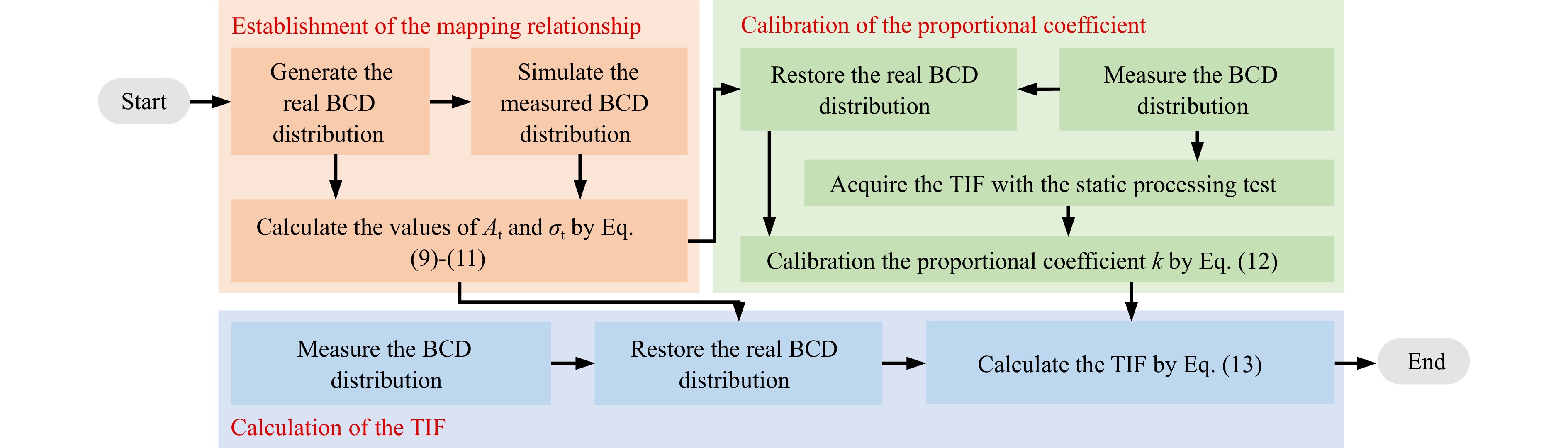
Fig. 6  Flowchart of the corrective measurement method for millimetre spot-sized TIF.

where d is the aperture diameter. Based on the above equations, the amplitude and FWHM both change in the measured BCD distribution, which is the critical error source of the FC measurement. To characterise this, two parameters, the amplitude reduction ratio $ {A_{\text{t}}} $ and FWHM expansion ratio $ {\sigma _{\text{t}}} $, are defined in Fig. 7. They are used to evaluate the convolution effect from two different perspectives, and can be expressed as follows:

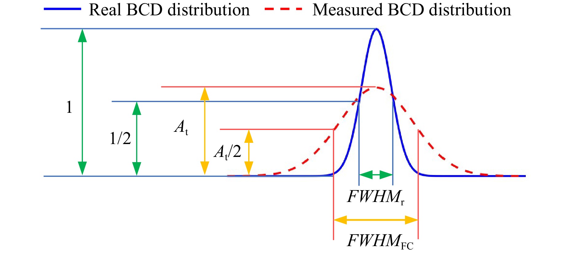
Fig. 7  Definition of the amplitude reduction ratio $ {A_{\text{t}}} $ and the FWHM expansion ratio $ {\sigma _{\text{t}}} $.

where $ FWH{M_{\rm r}} $ is the FWHM of the real BCD distribution. Considering the Sigmund theory, the value of $ FWH{M_{\rm r}} $ is considered to be same as the FWHM of the TIF. In the definition of the FWHM, the relationship between $ {A_{\rm t}} $ and $ {\sigma _{\rm t}} $ is represented by Eq. 11:

where $ {I_0}\left( {{{\sqrt {2\ln 2} r{\sigma _{\rm t}}} / \sigma }} \right) $ represents the modified Bessel function of the first kind. The detailed deduction is shown in the appendix. Thus, the closer the values of $ {A_{\rm t}} $ and $ {\sigma _{\rm t}} $ are to 1, the more closely does the measurement resemble the real BCD distribution, indicating a weaker convolution effect. Thus far, the changes in the measured BCD distribution can be described using these parameters. Using the aforementioned formula, the real BCD distribution can be defined and simulated to acquire the corresponding measured BCD distribution, thereby establishing a mapping relationship between the two distributions.

Thus, the parameter library with $ {A_{\rm t}} $ and $ {\sigma _{\rm t}} $ is established, which correspond with the values of $ FWH{M_{\rm r}} $ and $ FWH{M_{\rm{FC}}} $. In other words, based on the value of $ FWH{M_{\rm{FC}}} $ extracted from scanning, the values of $ {A_{\rm t}} $ and $ {\sigma _{\rm t}} $ can be determined, and in turn, the value of $ FWH{M_{\rm r}} $ in the TIF is directly obtained. However, the PRR of the TIF cannot be directly derived from $ {A_{\rm t}} $; it requires a unit transformation between the BCD and removal rate. Like the previous online measurement method, the proportional coefficient k has to be introduced through the static processing test, which is calculated as follows:

After the above two stages, when the FC scanning is conducted for any processing parameter, the values of k, $ {A_{\rm t}} $, and $ {\sigma _{\rm t}} $ can all be determined, rendering the accurate calculation of the TIF feasible. The final formula for the TIF is as follows:

Compared with Eq. 5, it is clear that the changes in the width and peak values are effectively compensated with the values of $ {A_{\rm t}} $ and $ {\sigma _{\rm t}} $ from the convolution effect, thereby enhancing the accuracy of the TIF measurement. The two key parameters proposed in this section are adequate to characterise the convolution effect, necessitating an analysis of only the parameter variations before and after convolution. In practical FC scanning, the noise interference has been effectively suppressed through point-by-point multi-frame averaging, resulting in highly smoothed measurement data that contribute to maintaining the accuracy of the two-parameter analysis. Thus, the proposed method eliminates the need for complex deconvolution processes, thereby significantly improving the computational efficiency.

With the definitions of $ {A_{\rm t}} $ and $ {\sigma _{\rm t}} $, this section provides a detailed analysis of the convolution effect. According to the formula derived in Section 3, the aperture and ion beam size can both influence the convolution effect, fundamentally because of their size ratio. Therefore, a calculation analysis was conducted to explore the influencing patterns by varying the aforementioned parameters following Eqs. 9-11. The value of $ {A_{\rm t}} $ was directly obtained from Eq. 9, following which the value of $ {\sigma _{\rm t}} $ was calculated using the iteration method with Eq. 11.

First, a single-factor analysis was carried out based on the two groups of parameters shown in Table 2, and the results are shown in Fig. 8. As shown in Fig. 8a, the decrease in $ FWH{M_{\text{r}}} $ causes $ {A_{\rm t}} $ and $ {\sigma _{\rm t}} $ to deviate further from 1, indicating a more pronounced convolution effect. Their variation trends are opposite, but both show a clear exponential trend. When $ FWH{M_{\text{r}}} $ exceeds 2 mm, the changes in $ {A_{\rm t}} $ and $ {\sigma _{\rm t}} $ occur at a slower pace. Moreover, Fig. 8b reveals that when $ {d_{{\text{FC}}}} $ is below a certain threshold, both $ {A_{\rm t}} $ and $ {\sigma _t} $ tend to approach 1. As $ {d_{{\text{FC}}}} $ increases, $ {A_{\rm t}} $ gradually decreases, while $ {\sigma _{\rm t}} $ gradually increases. Therefore, the changes in $ FWH{M_{\text{r}}} $ and $ {d_{{\text{FC}}}} $ have opposite impacts on the convolution effect.

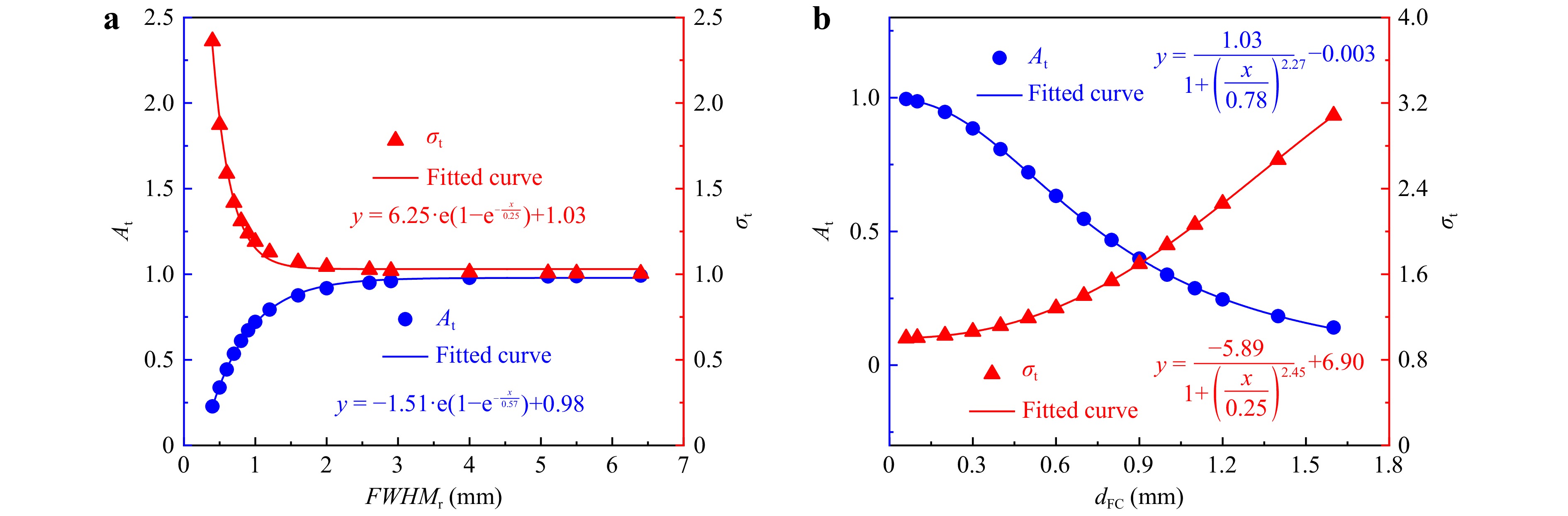
Fig. 8  Results of the calculation analysis. a Analysis of group 1. b Analysis of group 2.

To specifically analyse the impact of the beam-to-aperture size ratio on the convolution effect, the calculation analysis was further conducted using specific value combinations of $ {d_{{\text{FC}}}} $ and $ FWH{M_{\text{r}}} $. As shown in Table 3, when the size ratio is maintained, both $ {A_{\rm t}} $ and $ {\sigma _{\rm t}} $ are deterministic, indicating that the convolution effect remains consistent in this case. Therefore, the beam-to-aperture size ratio is the decisive factor in the convolution effect during FC measurement.

Based on this analysis, Fig. 9 further illustrates the changes in $ {A_{\rm t}} $ and $ {\sigma _{\rm t}} $ as the beam-to-aperture size ratio varies. It is clear that the convolution effect is progressively amplified as this size ratio decreases, presenting an exponential trend. These results explain the experimental results in Fig. 1 well. When the size ratio exceeds 3, $ {\sigma _{\rm t}} $ remains below 1.02 and $ {A_{\rm t}} $ remains around 0.96. At this point, both parameters are very close to 1, indicating that the convolution effect is already very weak. This implies that the convolution effect can be disregarded under this specific condition.

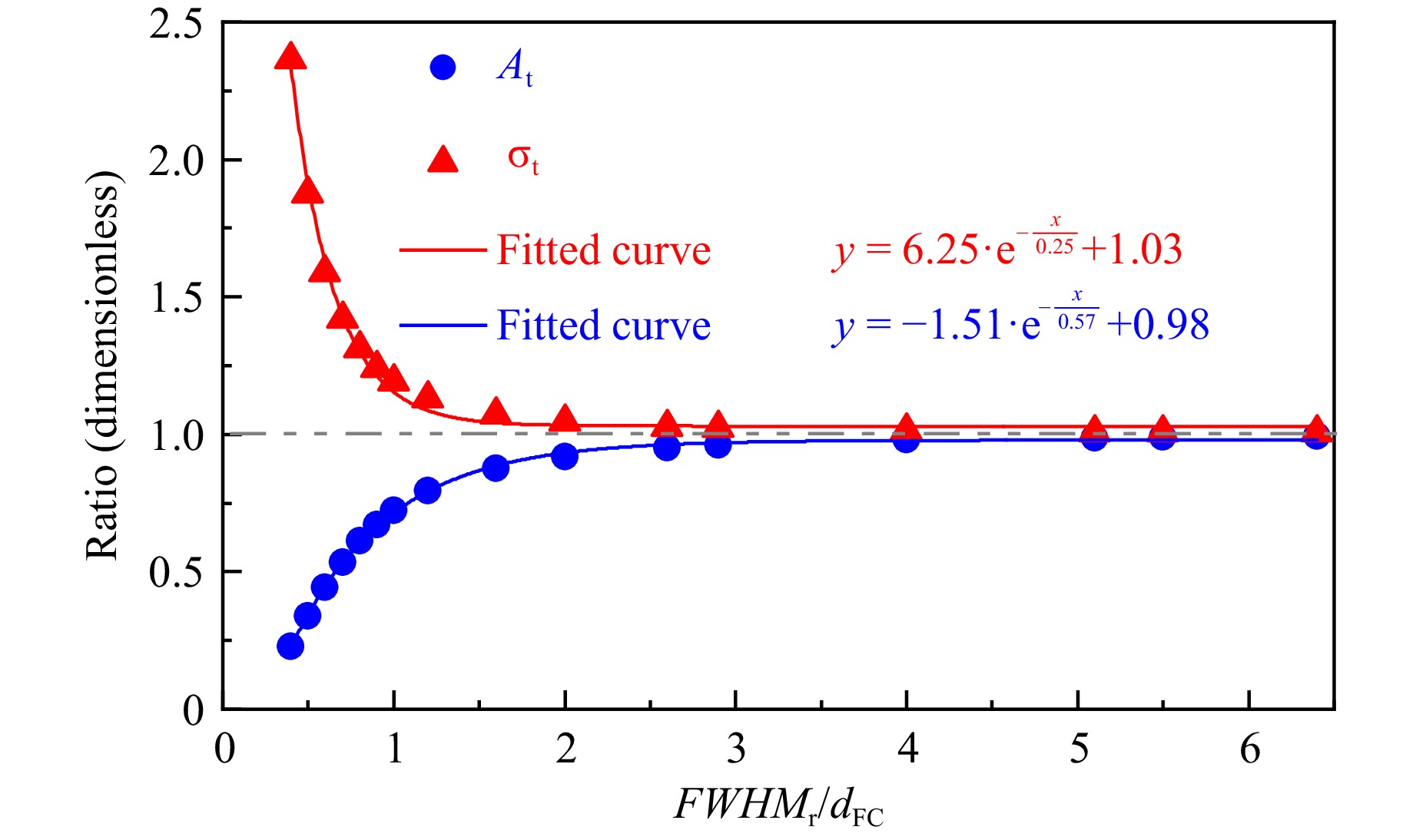
Fig. 9  Variations in $ {A_{\rm t}} $ and $ {\sigma _{\rm t}} $ with changes in the beam-to-aperture size ratio.

Fig. 10 provides a distribution analysis of three specific TIFs in Fig. 9. As the beam-to-aperture size ratio decreases, the measured BCD distribution deviates increasingly from the Gaussian type, as evidenced by a flatter top, which is highly consistent with the measurements in Fig. 1. Further, when the ratio decreases to a certain extent such that the diameter of the aperture is larger than the full width of the ion beam, the top of the measured BCD distribution is completely flat. Therefore, the impact of the convolution effect on the measurements is not limited to amplitude reduction and FWHM expansion, but also causes a deviation in the measured BCD distribution from the Gaussian type. Furthermore, as the ratio decreases, the convolution effect becomes more pronounced, and the degree of deviation from the Gaussian distribution increases.

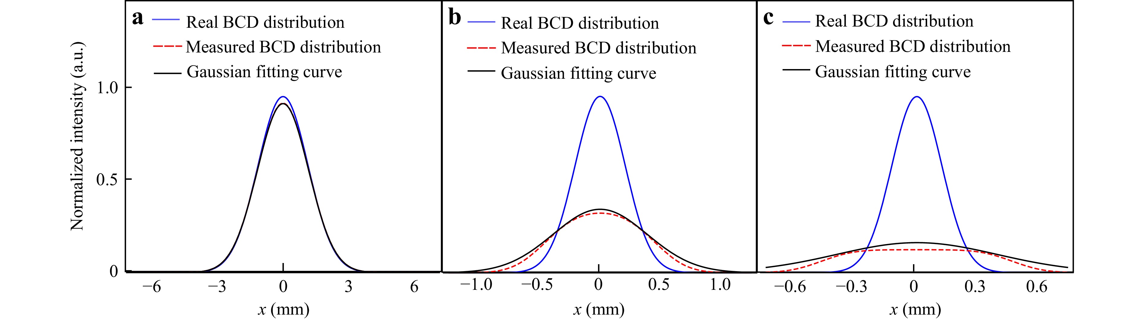
Fig. 10  Normalised comparison of the TIF distribution with different beam-to-aperture size ratios. a Size ratio of 3. b Size ratio of 0.5. c Size ratio of 0.3.

This section discusses a series of experiments carried out to verify the corrective measurement method for the small-sized TIF. The FC had an aperture of diameter 1 mm in this study. The experimental data were derived from Section 2, and all data pertained to small-sized TIFs. Based on the values of FWHM_FC, the parameter library was primarily established based on the mapping relationship between $ {A_{\rm t}} $ and $ {\sigma _{\rm t}} $ for this aperture (Table 4), as it was required for the subsequent analysis.

Considering the experimental results, the values of k were calculated by two online measurement methods, which are described in detail in Sections 2 and 3. Combined with the Sigmund theory, it is not difficult to understand that the value of k should be theoretically constant, which is determined by the sputtering yield depending on the material characteristic. Therefore, by comparing the two curves, the two calculated values of k are very close. As shown in Fig. 11, without considering the convolution effect, k does not exhibit the expected constant trend, but rather shows an exponential trend similar to the calculation results in Section 4. The corrective method requires consideration of the convolution effect, where k fluctuates within a small range around a constant value, aligning with the predictions of the Sigmund theory.

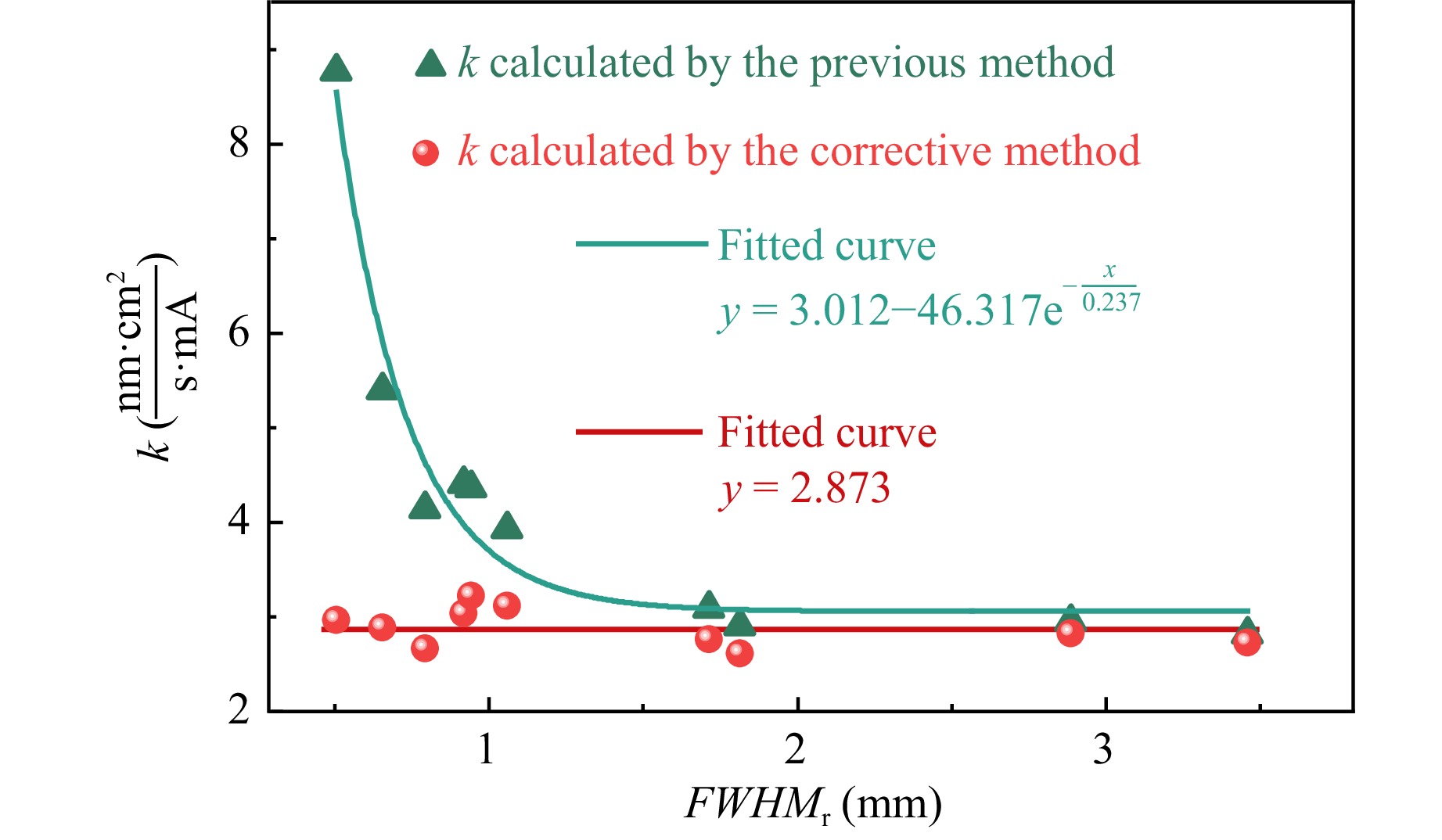
Fig. 11  Comparison of k obtained by two measurement methods.

With the calibrated k from the two methods, three TIFs with relatively smaller FWHMs were selected and calculated. Table 5 and Fig. 12 show the measurement errors in the PRR and FWHM, demonstrating a noticeable decrease in these errors when accounting for the convolution effect. Specifically, the average error in the PRR drastically decreases from 47.4% to 3.1%, while that in the FWHM decreases from 51.7% to 2.6%. Further, as can be observed intuitively from Fig. 12, the smaller the TIF, the more remarkable the improvement in the measurement accuracy using the corrective method.

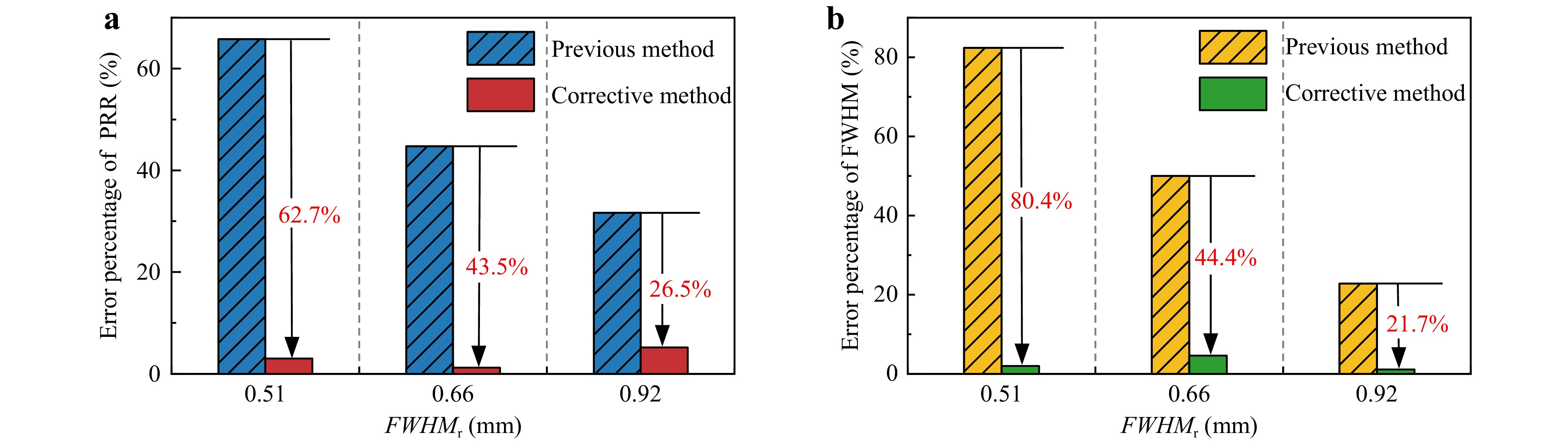
Fig. 12  Comparison of the two measurement methods. a Error percentage of the PRR. b Error percentage of the FWHM.

Fig. 13a compares the TIFs obtained from the two methods with an FWHM_r of 0.99 mm, demonstrating the remarkable accuracy of the corrective method. However, there still exists a certain measurement error in this method, which primarily manifests as a slightly larger FWHM compared to the real data. Based on the definition of $ {\sigma _{\rm t}} $, the FWHM from the experimental results presented in Section 2 is analysed in Fig. 13b, revealing that the experimental $ {\sigma _{\rm t}} $ is generally slightly larger than the theoretical value. This discrepancy is consistent with previous academic findings, where a small but consistent difference in the ion beam profile was obtained when the neutraliser was turned on and off. When the neutralizer is off, the ion beam tends to be wider³⁹; nevertheless, this discrepancy has a limited impact on the measurement results, making the calculations relatively reliable for practical polishing processes. Note again that the corrective measurement method is applicable to any optical material, but requires recalibration of the proportional coefficient k.

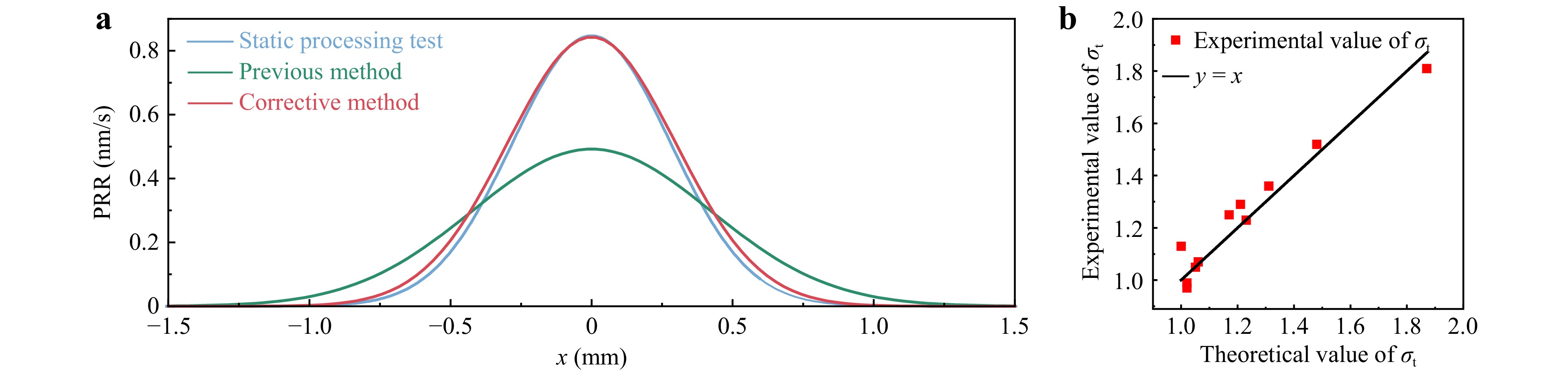
Fig. 13  Difference in the FWHM between the corrective method and experimental results. a Comparison of the BCD distribution between the two measurement methods for an FWHM_FC of 0.99 mm. b Comparison of σ_t obtained experimentally and theoretically for the experimental results in Section 2.

To further investigate the polishing performance with the corrective and previous methods, a series of simulations were carried out to compare the results with the static processing test results. A sinusoidal dwell time map was defined to generate the removal distribution, which uses the TIFs obtained by the different measurement methods. Specifically, the step size was 0.05 mm and the sinusoidal period was 2 mm. To analyse the theoretical convergence rate, the removal distribution obtained by convolving the TIF from the static processing tests with the dwell time map was defined as the target removal distribution. The simulation is achieved using the TIF with an FWHM_r of 0.51 mm, which is the smallest value for the static processing test in Table 2 (Fig. 14).

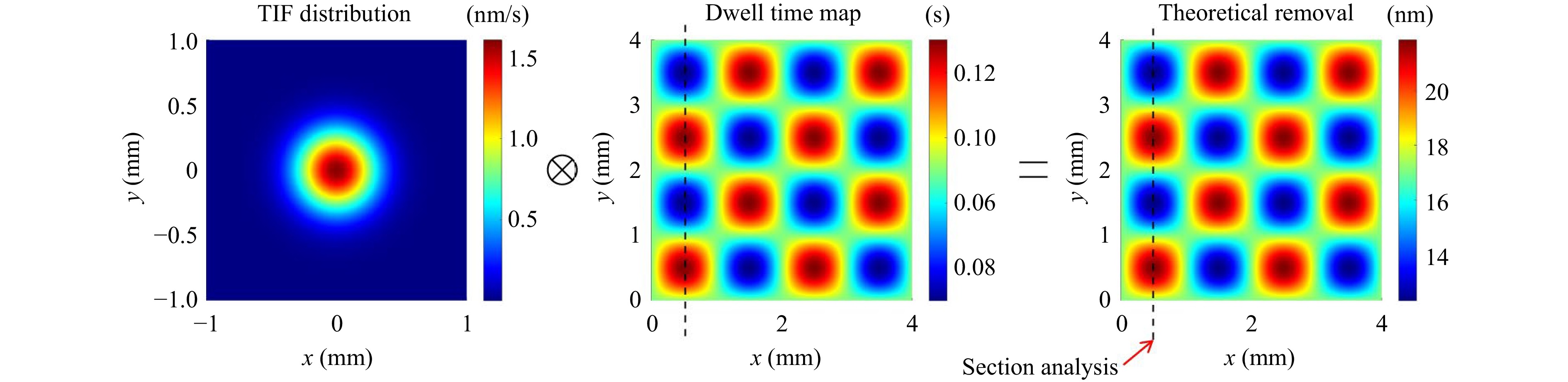
Fig. 14  Simulation procedure for the TIF with an FWHM_r of 0.51 mm.

Fig. 15 and Table 6 show the simulation results for the aforementioned three groups of TIFs, which are compared with the corresponding static processing test results. The section position is illustrated in Fig. 14, and the root-mean-square (RMS) value is used to describe the form errors. For the previous method shown in Fig. 15b, d, f, there exists a notable processing error between the target and practical removal distributions. Comparatively, the simulation results with the corrective method are more accurate, as shown in Fig. 15a, c, e. For TIFs with the FWHM ranging from 0.5 to 1 mm, the average theoretical convergence rate improves from 48.0% to 95.3%.

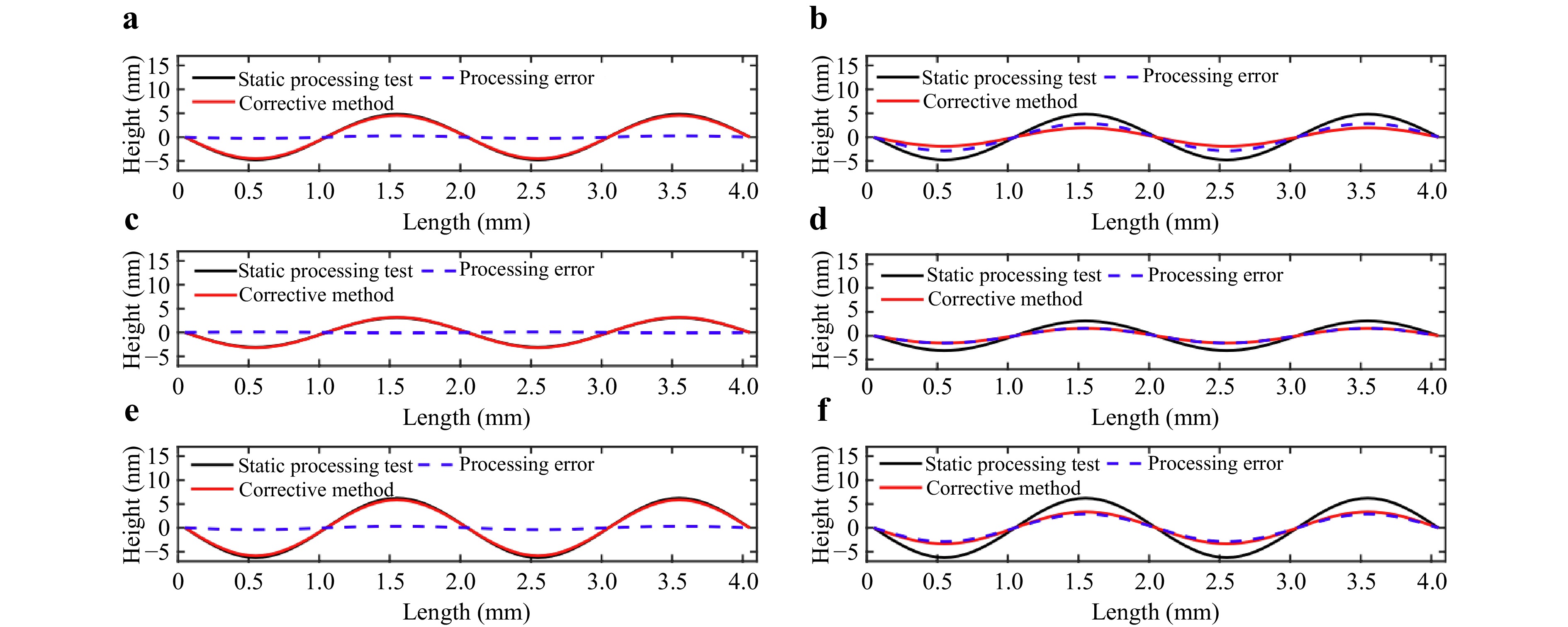
Fig. 15  Comparison of the simulation results for removal distributions with different TIFs. a Corrective measurement method with an FWHM_r of 0.51 mm. b Previous measurement method with an FWHM_r of 0.51 mm. c Corrective measurement method with an FWHM_r of 0.66 mm. d Previous measurement method with an FWHM_r of 0.66 mm. e Corrective measurement method with an FWHM_r of 0.92 mm. f Previous measurement method with an FWHM_r of 0.92 mm.

To validate the practicality of the corrective measurement method, the polishing experiment was conducted on an aspherical optical mirror with a clear aperture of approximately 500 mm, and the RMS value was 1.7 nm. The experiment was conducted using the parameters of the No. 8 TIF listed in Table 1, and the FWHM of the measured BCD distribution obtained from the FC was 1.90 mm. According to the corrective measurement method, the FWHM_r of the TIF was 1.81 mm, whereas with the previous method, it was 1.90 mm. Therefore, the target processing spatial wavelength was in the range of 15 mm to 3.6 mm.

First, the two TIFs were used to calculate the dwell time map and theoretical form error separately. Note that the actual processing results can be predicted by convolving the real TIF with these two dwell time maps separately. Based on the above experimental validation results, the TIF measured by the corrective method was sufficiently accurate; hence, it was considered the real TIF. Fig. 16a, b compares the dwell time maps using different measurement methods. The total dwell time with the corrective method is 47.3 h, while that with the previous method is 42.1 h. The form errors after theoretical processing based on the two dwell time maps are shown in Fig. 16. The RMS of the corrective method is approximately 0.1 nm, while that obtained with the previous method is approximately 0.2 nm, and the corresponding theoretical convergence rates are 94.1% and 88.2%, respectively.

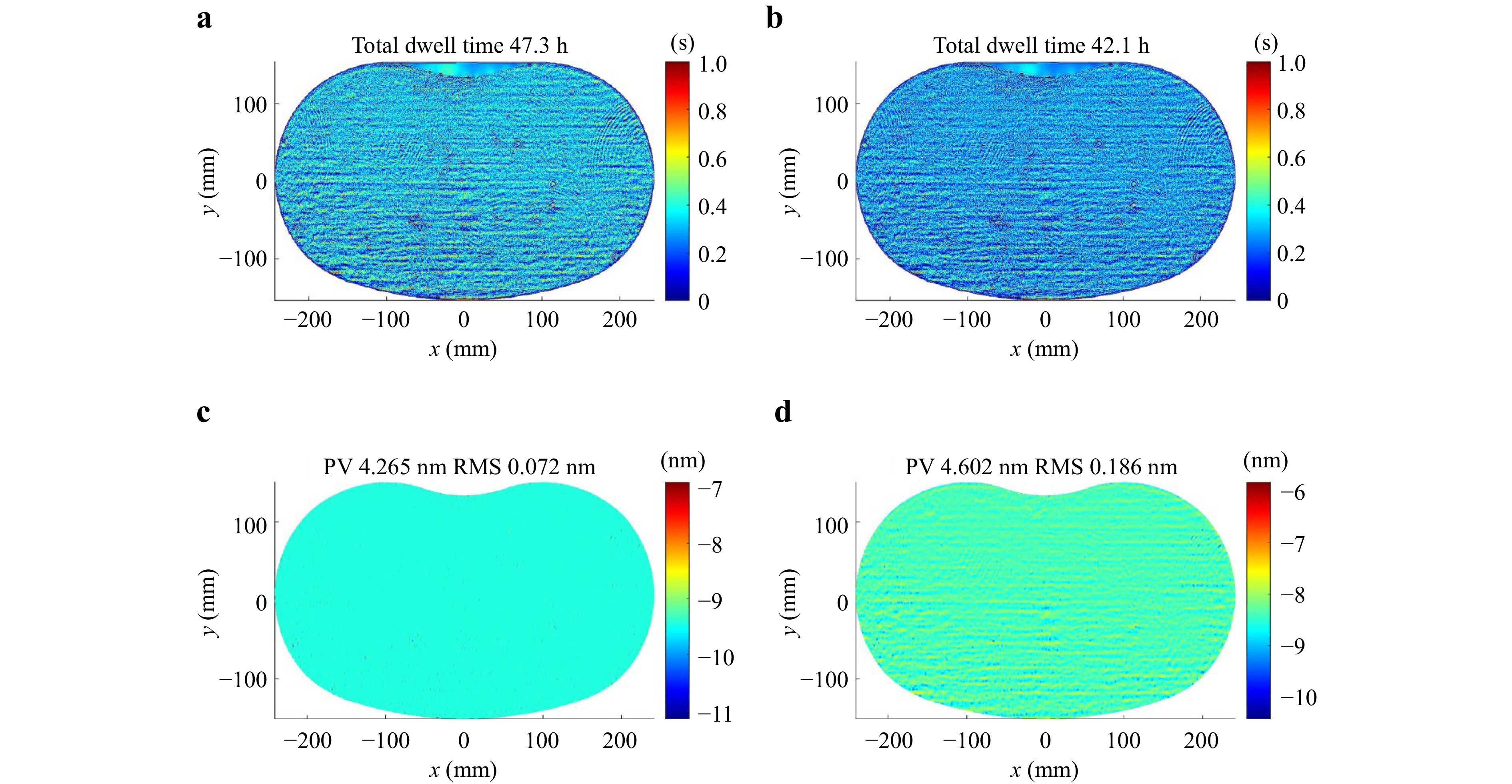
Fig. 16  Comparison of the dwell time maps and processing results. a Dwell time map of the corrective measurement method. b Dwell time map of the previous measurement method. c Processing result of the corrective measurement method. d Processing result of the previous measurement method.

The RMS density (RMSD) is used to describe changes in the form errors at different spatial wavelengths (the reciprocal of the spatial frequency) before and after processing. The RMSD serves as an efficient metric to describe the power spectral density (PSD) of a two-dimensional isotropic surface, as it provides both intuitive and quantitative insights into form errors across different spatial wavelengths⁴⁰. Equation 14 is widely used to define the RMSD and express its relationship with the PSD⁴¹.

where α is the decadic number. The theoretical convergence rate analysis results based on the RMSD are shown in Fig. 17. Within the target spatial wavelength range, the theoretical average convergence rate of the corrective method reaches 98.4%, which is higher than that with the previous method (90.1%). Thus, the corrective method yields better processing results, and considering its practicality, it was used in the experiment.

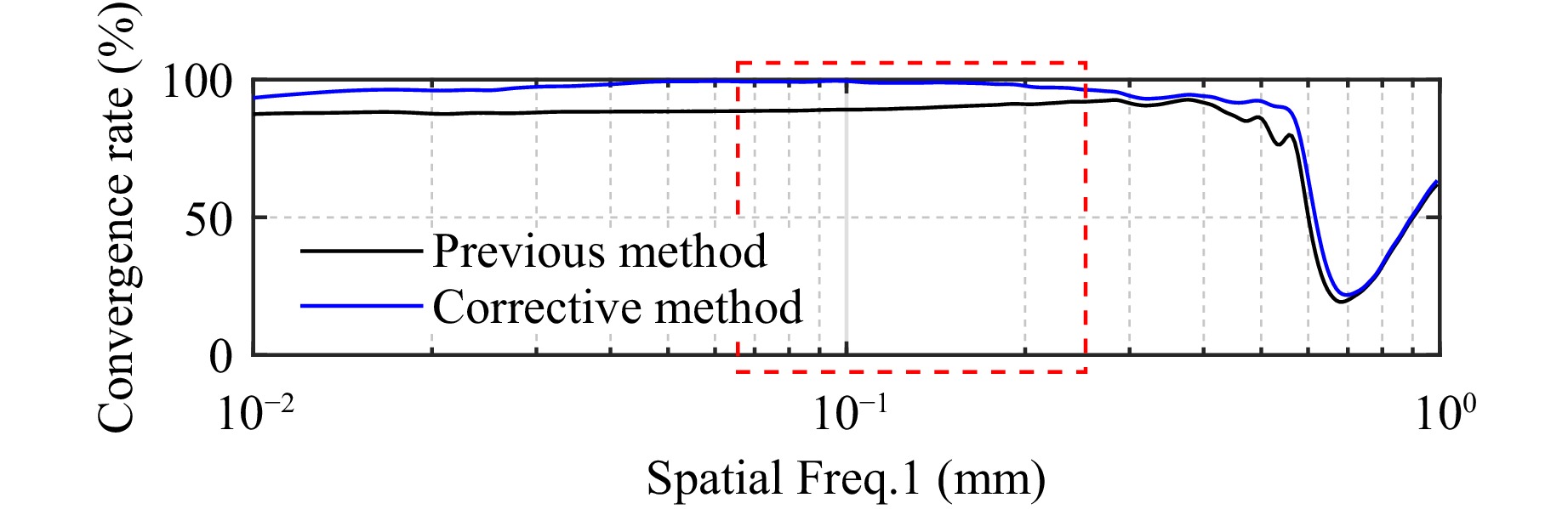
Fig. 17  Comparison of the RMSD curves of form errors using different measurement methods.

Fig. 18 shows a photograph of the experimental setup for the polishing experiment. The form errors before and after processing are shown in Fig. 19; the figure indicates that the RMS of the aspherical optical mirror decreases from 1.7 nm to 0.4 nm. The actual convergence rate is 76.5%, which is lower than the theoretical expectation of this method, mainly due to factors such as the fluctuation in the TIF and insufficient positioning accuracy during processing.

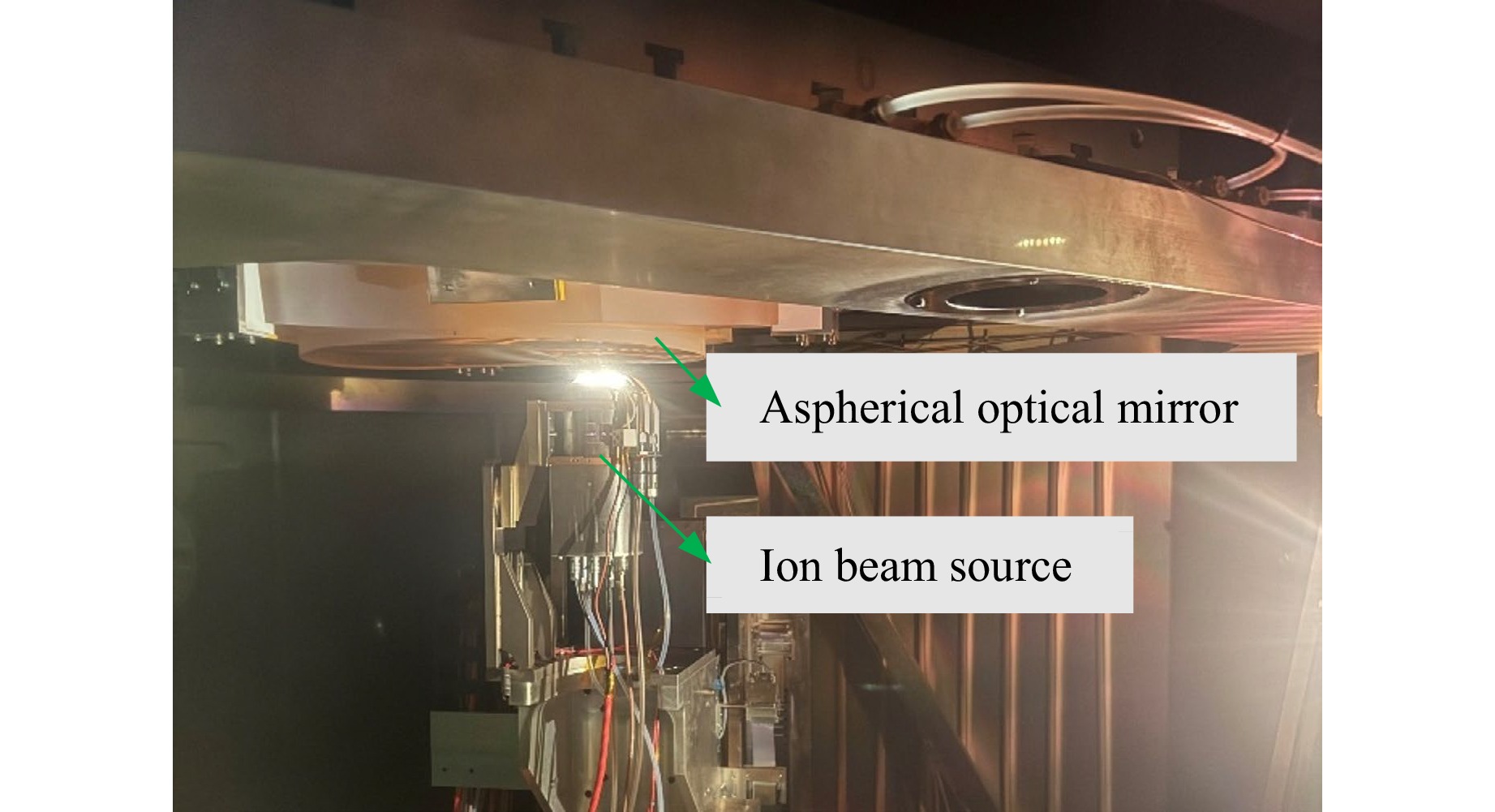
Fig. 18  Experimental setup for the polishing experiment.

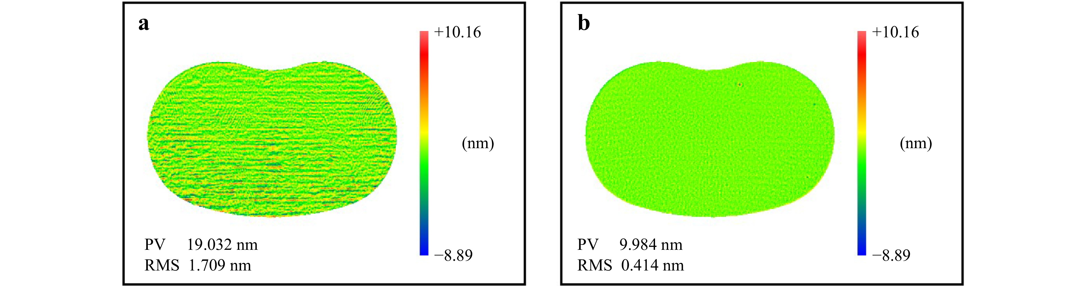
Fig. 19  Experimental results. a Form errors before processing. b Form errors after processing.

To investigate the changes in the convergence rate corresponding to different spatial wavelengths, the RMSD results of the form error before and after processing were analysed. According to Fig. 20a, the form errors within the target spatial wavelength range effectively converge. As shown in Fig. 20b, the convergence rate varies from 47.0% to 90.7% and the actual average convergence rate is 76.4%. Compared to Fig. 17, in the lower-frequency domain, the actual convergence rate is close to or even surpasses the theoretical convergence rate of the previous method. Considering the difference between the actual and theoretical convergence rates of the corrective method, the actual convergence rate would be lower with the previous method. The above results demonstrate the effectiveness of the proposed method in practical processing.

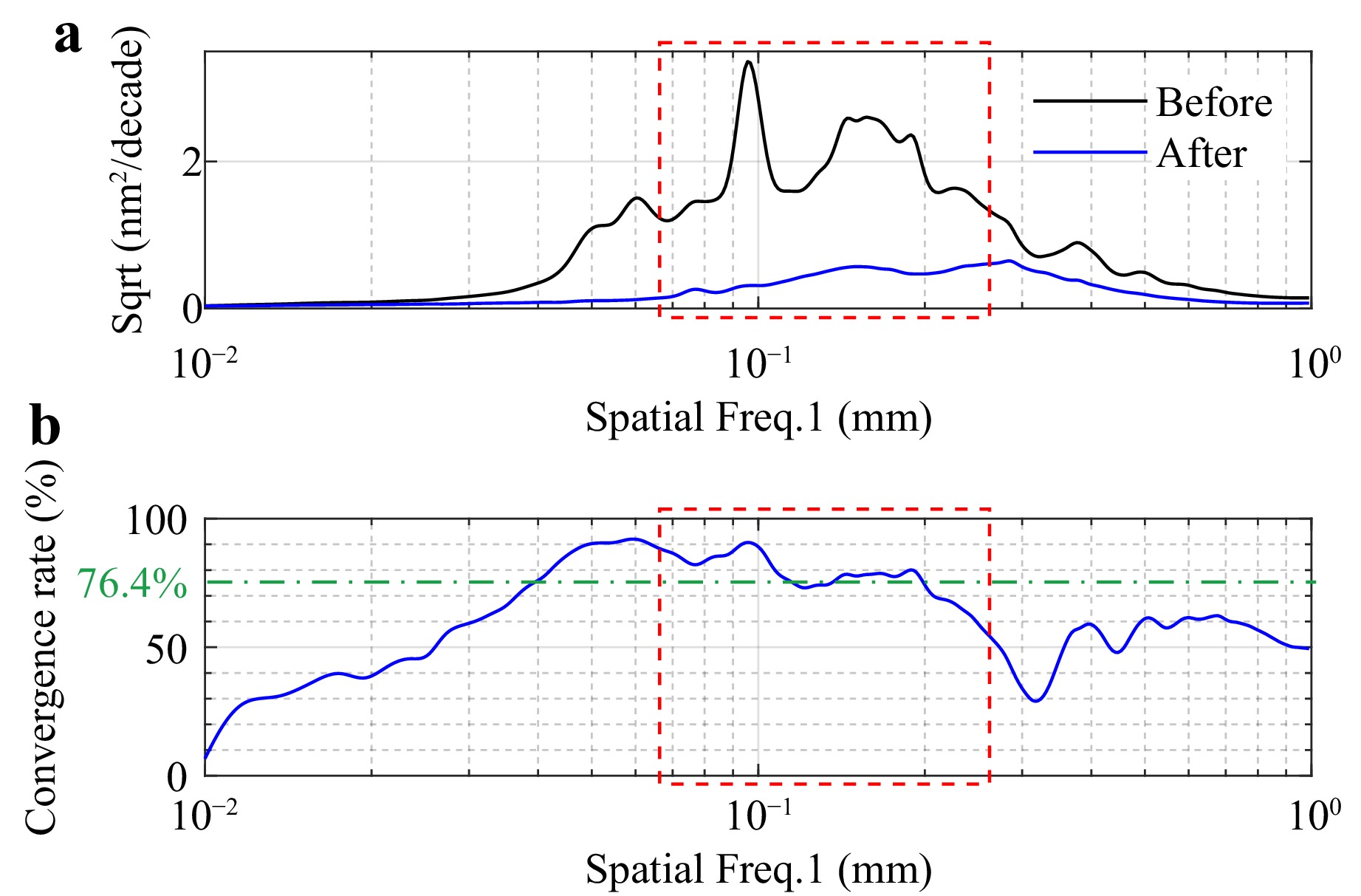
Fig. 20  Experimental results. a RMSD curves of form errors before and after processing. b Convergence rates at different spatial wavelengths.

In summary, the corrective online measurement method for millimetre spot-sized IBF exhibits high precision, effectively validating its accuracy. This method is universally applicable to the small-sized TIF measurements of optical elements, which can be used for the high-precision fabrication of optics.

According to Section 4, the corrective measurement method is crucial for small-sized TIFs. In the previous method, the convolution effect can be considerably mitigated by changing the beam-to-aperture size ratio, which reduces the discrepancy between the measured and real BCD distributions. Thus, by optimising the size ratio, the previous method may also be feasible for measuring small-sized TIFs. In practice, this can be achieved by reducing the aperture of the FC. To investigate this, the experiment was designed to compare the two methods, and the experimental parameters are shown in Table 7. The experimental conditions are consistent with those described in Section 2. With this experimental design, we obtained TIFs with FWHM_r values ranging from 0.5 mm to 0.8 mm.

The experimental results are presented in Fig. 21, Fig. 22, and Table 8. After parameter optimisation, the previous method achieves an average FWHM measurement error of approximately 10% for small-sized TIFs, surpassing unoptimized outcomes. This highlights the effectiveness of enhancing the measurement accuracy through aperture diameter reduction. However, notable deviations in the PRR measurements are observed. This is primarily due to the significant reduction in the aperture area, which causes a substantial decrease in the instantaneous current, thereby posing challenges to current resolution of the FC. Other factors, such as background noise, may also have influenced the measurements. By contrast, the corrective measurement method demonstrates a clear advantage in terms of accuracy, achieving more precise measurements for both the FWHM and PRR.

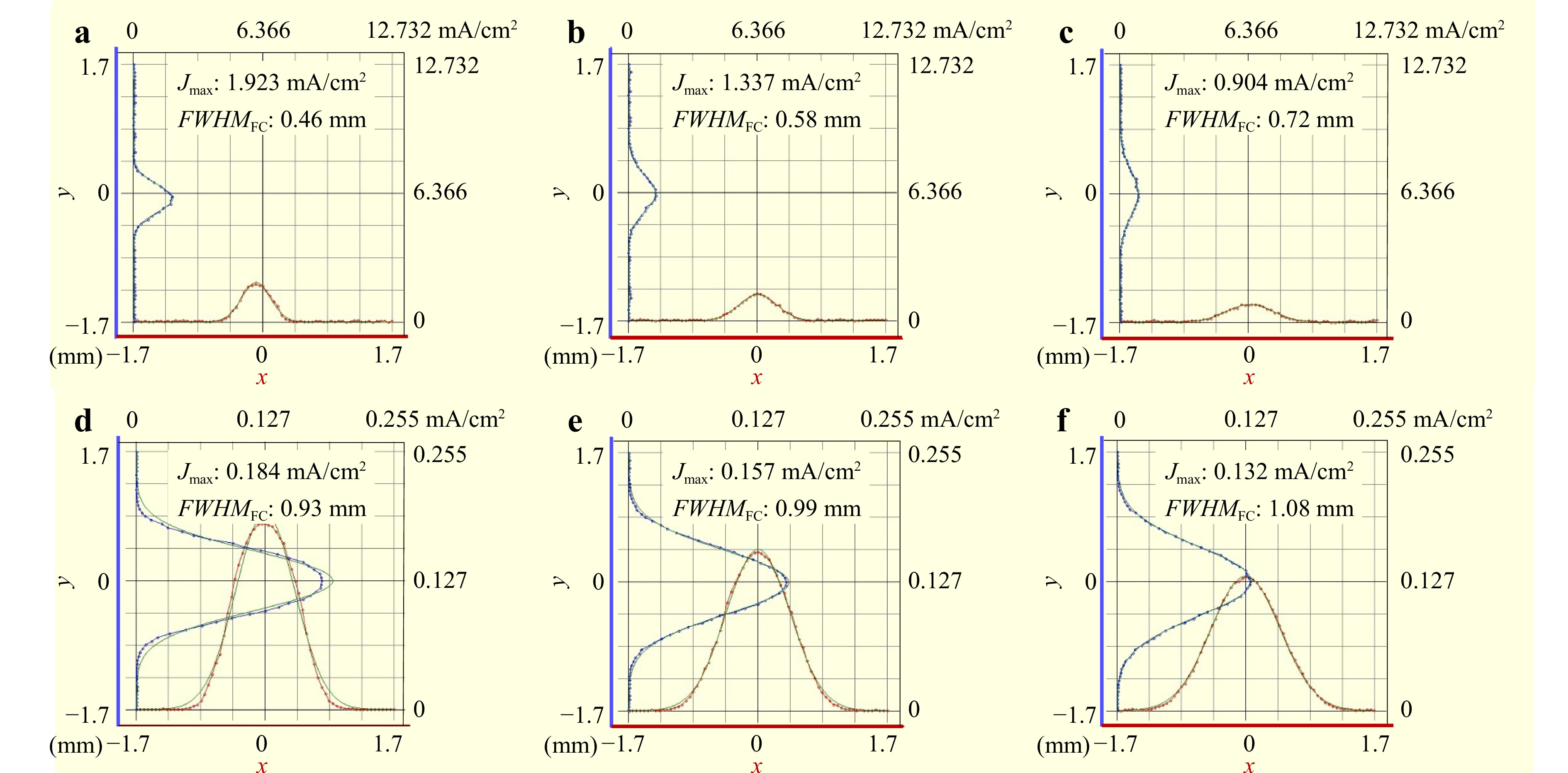
Fig. 21  a-c FC measurements of group 3. d-f FC measurements of group 4.

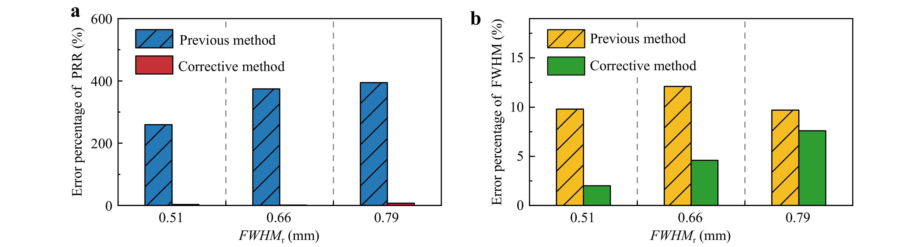
Fig. 22  Comparison of the two measurement methods. a Error percentage of the PRR. b Error percentage of the FWHM.

While the convolution effect can be theoretically mitigated by optimising the parameters, the previous method still cannot be used to measure small-sized TIFs with high accuracy. The measurement error cannot be fundamentally solved, and there are also other issues. In summary, the corrective method is indispensable for the online measurement of small-sized TIFs.

In the high-precision fabrication of short-wavelength optics, millimetre spot-sized IBF is an effective process for eliminating form errors with spatial wavelengths ranging from 10 to 1 mm. To achieve this, the precise measurement of small-sized TIFs (with an FWHM below 2 mm) is imperative. However, a significant convolution effect occurs in the FC measurement when the beam size is close to the aperture size. Therefore, the existing online measurement method is not sufficiently accurate for small-sized TIFs. To overcome this, a calculation analysis is mathematically conducted in this paper. The findings show that the convolution effect grows stronger with a decrease in the beam-to-aperture size ratio. This effect not only manifests as exponential variations in the measured FWHM and amplitude, but also in the form of increasing deviation of the measured BCD distribution from the Gaussian shape. Based on this, a corrective online measurement method is proposed in this paper. As confirmed by experiments, the corrective measurement method exhibits a higher precision than the previous method. For TIFs with FWHMs ranging from 0.5 to 1 mm, the average error of the PRR is reduced from 47.4% to 3.1%, and the average error of the FWHM is reduced from 51.7% to 2.6%. These improvements can enhance the average theoretical convergence rate, which is necessary for the high-precision fabrication of optics. By applying this method to a polishing experiment, a high-precision aspherical optical mirror is obtained with an RMS of 0.4 nm, and the actual average convergence rate is 76.4% within the target spatial wavelength range of 15 mm to 3.6 mm. Owing to practical implementation issues, the previous measurement method was rendered inapplicable, even though a reduction in the size of the aperture can theoretically mitigate the impact of the convolution effect. Therefore, the proposed corrective measurement method is necessary for the rapid and precise measurement of small-sized TIFs, as it can facilitate the modulation of the TIF and enable real-time monitoring of its stability. This proposed method is indispensable for millimetre spot-sized IBF, and can meet the requirements for the high-precision fabrication of optics.

The work was supported by National Natural Science Foundation of China (62127901, 12103054, 62405314, 62305333, 62375260); National Key Research and Development Program of China (2022YFB3403405); Scientific and Technological Development Program of Jilin (SKL202402021); Youth Innovation Promotion Association of the Chinese Academy of Sciences (2019221, Y2023062); Youth Elite Scientists Sponsorship Program of CAST (2022QNRC001); Young Elite Scientists Sponsorship Program of Jilin Province (QT202222); Scientific and Technological Program of Changchun (2024GZZ19).