


HTML
-
Since its emergence in the 1990s, multi-photon 3D direct laser writing (DLW), also known as 3D laser printing, has evolved from a scientific curiosity to an important 3D micro- and nanofabrication technique1, 2. Today, applications range from metamaterials3, 4 and biomimetics5 to microoptical components6, 7 and photonic interconnects8, 9.
However, challenges exist in that the physical 3D microstructures obtained from 3D printing often differ significantly from the underlying 3D computer models. Typically, shape distortions of readily printed 3D microstructures can, for example, result from the proximity effect10, volume shrinkage of the polymerised photoresist during polymerisation11, sample development12, or from a limited printing resolution13. Therefore, the 3D printing process must usually be optimised iteratively until the targeted 3D structure is reproduced with the required accuracy and quality. To date, this optimisation procedure has typically been based on imaging techniques, such as scanning electron microscopy14, holographic tomography15, X-ray tomography16, confocal fluorescence microscopy17, 18, confocal laser profilometry19, optical coherence tomography20, 21 and atomic force microscopy22.
These methods are carried out on the finished 3D printed parts using ex-situ approaches, that is, after the unpolymerised photoresist has been washed out using organic solvents. Hence, the optimisation processes relying on such ex-situ methods are comparatively slow.
An in-situ inspection method routinely used in the context of DLW is wide-field optical microscopy. Herein, one observes two-dimensional snapshots of light scattering from the momentary refractive-index distribution due to the unpolymerised and polymerised parts23. Reconstruction of the overall polymerised 3D microstructure from these data points is presently elusive and perhaps not even conceptually possible without deriving the phase or intensity information from the image. Another in-situ approach is coherent anti-Stokes Raman scattering (CARS) microscopy24, which allows for a spectroscopic determination of the local cross-linking density. However, this approach is relatively slow and cannot be used as a routine on-the-fly diagnostic tool. Thus, non-invasive in-situ 3D monitoring techniques that enable a fast and routine identification of printing defects during the printing process are missing to date. For example, X-rays would polymerise the monomer around the already printed (polymerised) regions and would therefore completely change the part to be inspected.
An ideal in-situ imaging modality should 1) be fast with respect to the printing process, so that the monitoring does not significantly increase the printing time; 2) give at least micrometer-scale 3D resolution; and, importantly, 3) not influence the printing process, i.e., not introduce any polymerisation or other unwanted chemical modifications of the photoresist.
Optical coherence tomography (OCT) is a promising candidate for in-situ inspection during multi-photon 3D laser printing. OCT relies on the interferometric detection of backscattered light from a sample. In the scope of in-situ DLW process monitoring, backscattering from the sample occurs because of the very small refractive-index differences between the polymerised and unpolymerised regions in the photoresist on the scale of
$ \Delta n \approx 10^{-2} $ and below25. Fourier-domain OCT systems can combine fast acquisition speeds and micrometer-scale resolution26 with high sensitivities exceeding$ 100 $ dB and are hence able to detect such small refractive index differences. Finally, polymerisation of the monomer used for printing by an OCT light source is obviously unwanted. For printing via two-photon absorption, we use tightly focused mode-locked femtosecond laser pulses centred at around$ 780 $ nm wavelength. Therefore, a continuous-wave OCT light source at a similar wavelength does not lead to two-photon or one-photon absorption. However, a continuous-wave OCT light source with significant power at approximately half of the 780 nm wavelength polymerises the monomer by one-photon absorption. Various continuous-wave OCT light sources are potentially compatible with these conditions. We choose superluminescent diodes, which are compact, readily available with similar wavelengths as the printing laser, and provide sufficiently large emission powers in the range of a few milliwatts.In the context of other 3D printing methods, in-situ 3D diagnostics using OCT have already been demonstrated in combination with extrusion-based bioprinting27, 28. Using gauging software, deviations from the original 3D computer model were revealed in a 3D OCT reconstruction. Furthermore, several studies on metal additive manufacturing used OCT for the in-situ monitoring of surface defects, layer roughness, and time-dependent thickness of the sintered metal29-31. In addition, the use of OCT for visualising the curing process in semi-transparent polymer droplets has been described recently32.
In this paper, we examine and demonstrate the feasibility of Fourier-domain optical coherence tomography (FD-OCT) as an in-situ diagnostic tool for multi-photon 3D laser printing. We start with OCT imaging of photoresists before 3D printing. Next, we investigate the polymer-substrate interface and the polymer-monomer interface of the printed structures. Thereafter, OCT imaging is applied to various 3D example architectures. To mimic the in-situ situation, these architectures are examined after laser printing, but before development. Several structures are inspected after development, followed by re-immersion in the same photoresist. We observe a time-dependent behaviour of the reflectivity at the polymer-monomer interfaces, which we model using graded-index profiles and a transfer-matrix approach. Subsequently, we examine the effective numerical aperture of our setup on a custom-printed 3D test target. Finally, we discuss the influence of different printing process parameters on the imaging contrast and show the OCT reconstructions recorded for a variety of 3D printed microstructures.
-
The scheme of our custom-built OCT apparatus is outlined in Fig. 1a. Low-coherence light is emitted from a fibre-coupled superluminescent diode (SLD, Exalos EXC250002-00) with a centre wavelength of
$ 845 $ nm, nominal full width at half maximum (FWHM) of$ 135 $ nm, and coherence length of$ 3.1 $ μm in air. A measurement of the intensity spectrum emitted by the SLD is shown in Fig. 1b. The light path is then split into reference and sample arms using a 50:50 fibre coupler (FC). The reference arm (bottom) consists of a fibre collimator (CL), an optical relay, and a reference mirror (RM). To obtain the highest possible OCT dynamic range without saturating the spectrometer line-scan detector, a neutral density filter (NDF) is used for optimising the intensity of the reference arm with respect to that of the sample arm.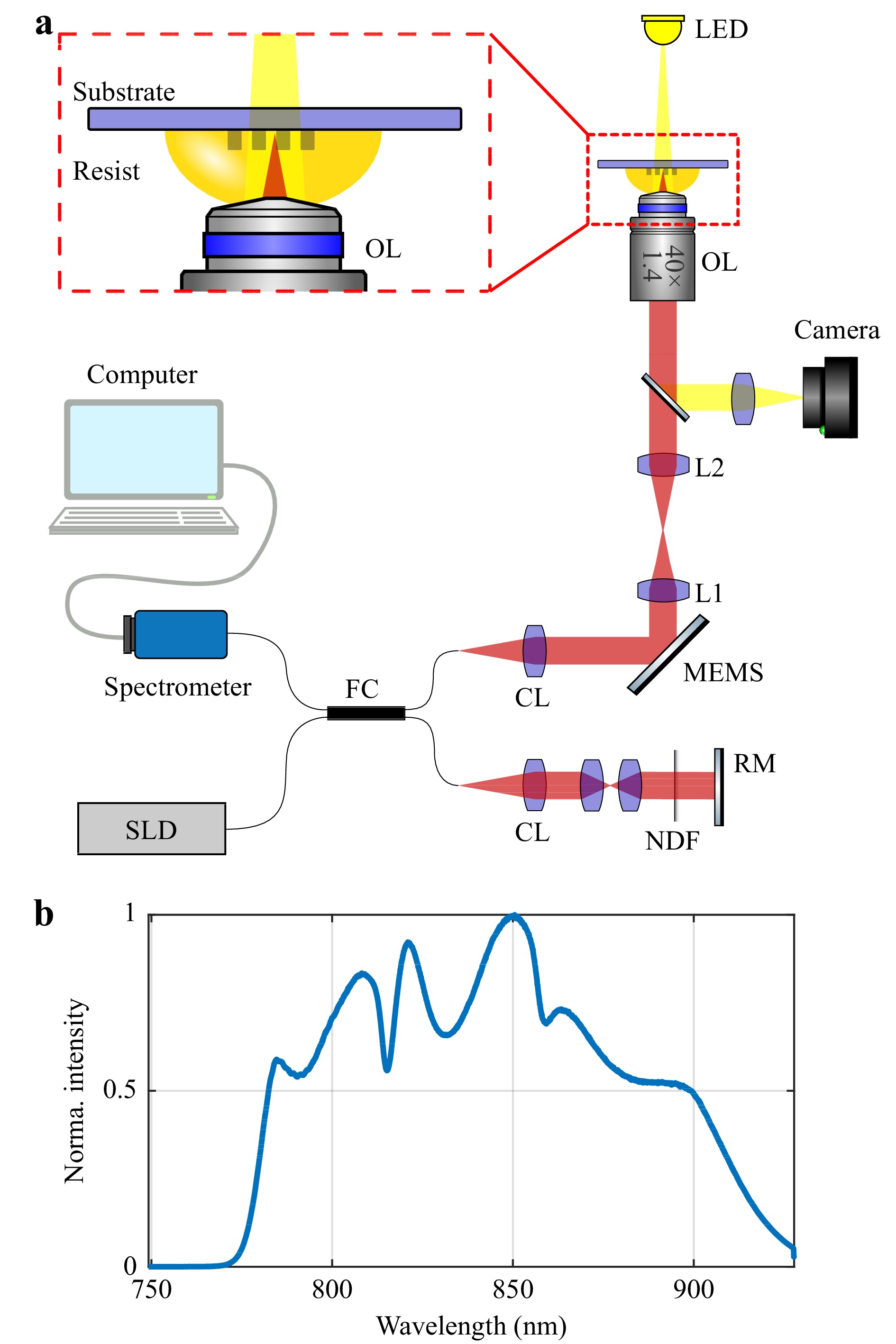
Fig. 1 Experimental FD-OCT setup. a Near-infrared low-coherence light (red path) is emitted from a superluminescent diode (SLD). After passing the 50:50 fibre coupler (FC), the emission is split into two arms. The reference arm (bottom) consists of a fibre collimator (CL), an optical relay and a reference mirror (RM). A neutral density filter (NDF) is used to optimize the intensity of the reference arm with respect to that of the sample arm. The light in the sample arm (top) is scanned using a MEMS mirror, then passes through the beam expander (L1 and L2) and is focused into the sample by an immersed objective lens (OL). The transmission illumination path is drawn in yellow. The spectral interference between the two arms is recorded by a spectrometer. This overall beam path could be combined with that of a two-photon laser printer along the same optical axis and using the same microscope objective lens. Alternatively, the beam path could be added to the printer from the other side of the glass substrate, requiring two objective lenses (also, see Supplementary Information Figure S1). b Measured intensity spectrum of the SLD.
The sample arm is set up such that the setup mimics the situation of an OCT system integrated into a state-of-the-art 3D laser-printing setup. Specifically, we use an immersion high-numerical-aperture lens, which is also commonly used for printing. After the light is coupled to free space using a fibre collimator, the beam is scanned using a two-axis MEMS mirror (Mirrorcle A5M24.2-2400AL). To obtain the targeted lateral OCT resolution, the beam is then expanded by a factor of
$ 1.2 $ using two achromatic doublets, resulting in a$ 1/e^2 $ beam diameter of$ 1.2 $ mm entering the immersion objective lens (Plan Apochromat 40x/1.4 DIC M27, Carl Zeiss), and focusing the light into the sample. An additional wide-field visual inspection of the sample is performed using a CCD camera (Flir Blackfly BFLY-PGE-50H5M) and an illumination LED ($ \lambda = 580 $ nm), which is coupled out of the beam path using a long-pass dichroic mirror (Thorlabs DMLP650).Particular attention should be paid to the objective lens. If one focuses into the sample using a large numerical aperture (NA), the axial field of view that can be imaged within one A-scan is limited, which is undesirable for the inspection of tall specimens. This is because the axial response of the OCT system can be described by a convolution between the coherence gate function and the confocal gate function33. For a large NA common for immersion objectives, confocal gating significantly reduces the axial field of view and causes the imaging system to begin operating in the optical coherence microscopy regime34. In this regime, the imaging system can only acquire en face tomographic images that are unsuitable for fast 3D reconstruction. Thus, we under-illuminate the back aperture of the objective lens, reducing its nominal numerical aperture from
$ \mathrm{NA} = 1.4 $ (used for laser printing) to an effective$ \mathrm{NA}_\mathrm{eff} = 0.22 $ (used for OCT imaging). This choice leads to an OCT axial field of view (OCT imaging depth) of up to$ 1 $ mm. As a side effect, the lateral resolution is reduced to approximately$ 1.9 $ μm. The axial resolution of OCT does not depend on the numerical aperture of the objective lens.Finally, the resulting interferogram is recorded using a fibre-coupled spectrometer with a line-scan detector (Wasatch Photonics CS800-840/180). To evaluate the recorded spectra, we perform standard FD-OCT data analysis procedures with home-built MATLAB software that includes resampling to k-space, dispersion compensation26, Hann windowing, zero padding, and fast Fourier transform (FFT). It takes approximately 30 s for a regular workstation to acquire (10 s) and process (20 s) the whole volumetric data corresponding to an exemplary volume of 400 μm × 400 μm ×2.6 mm (i.e., 500 × 500 A-scans with 40 μs for one A-scan). Printing a sample filling of this volume takes more than two orders of magnitude longer than 30 s. Therefore, one could interrupt the printing process a couple of times to obtain in-situ OCT data and then proceed as planned or modify the printing process without extending the overall printing time much.
We begin by validating our setup on planar samples with immersion, as depicted in Fig. 2. In Fig. 2a, we plot two A-scans recorded on a reflective surface (fused silica substrate in immersion oil, Immersol 518F, Carl Zeiss AG) with and without employing Hann windowing of the recorded spectrum. Hereafter, the phrase “OCT signal” refers to the absolute value of the Fourier transform and the phrase “OCT intensity” refers to a squared OCT signal. Throughout this paper, we normalise the OCT signal such that 0 dB corresponds to a 100% reflectivity for both the OCT signal and the OCT intensity. In particular, for an A-scan without Hann windowing, we deduce an FWHM of 2.1 μm, which is consistent with the SLD coherence length in immersion oil (2.05 μm) and represents the axial point-spread function of the OCT apparatus. However, for the sake of suppressed side lobes, we use Hann windowing, which increases the axial FWHM to 2.7 μm. A typical B-scan of the same substrate on a logarithmic scale is presented in Fig. 2b.
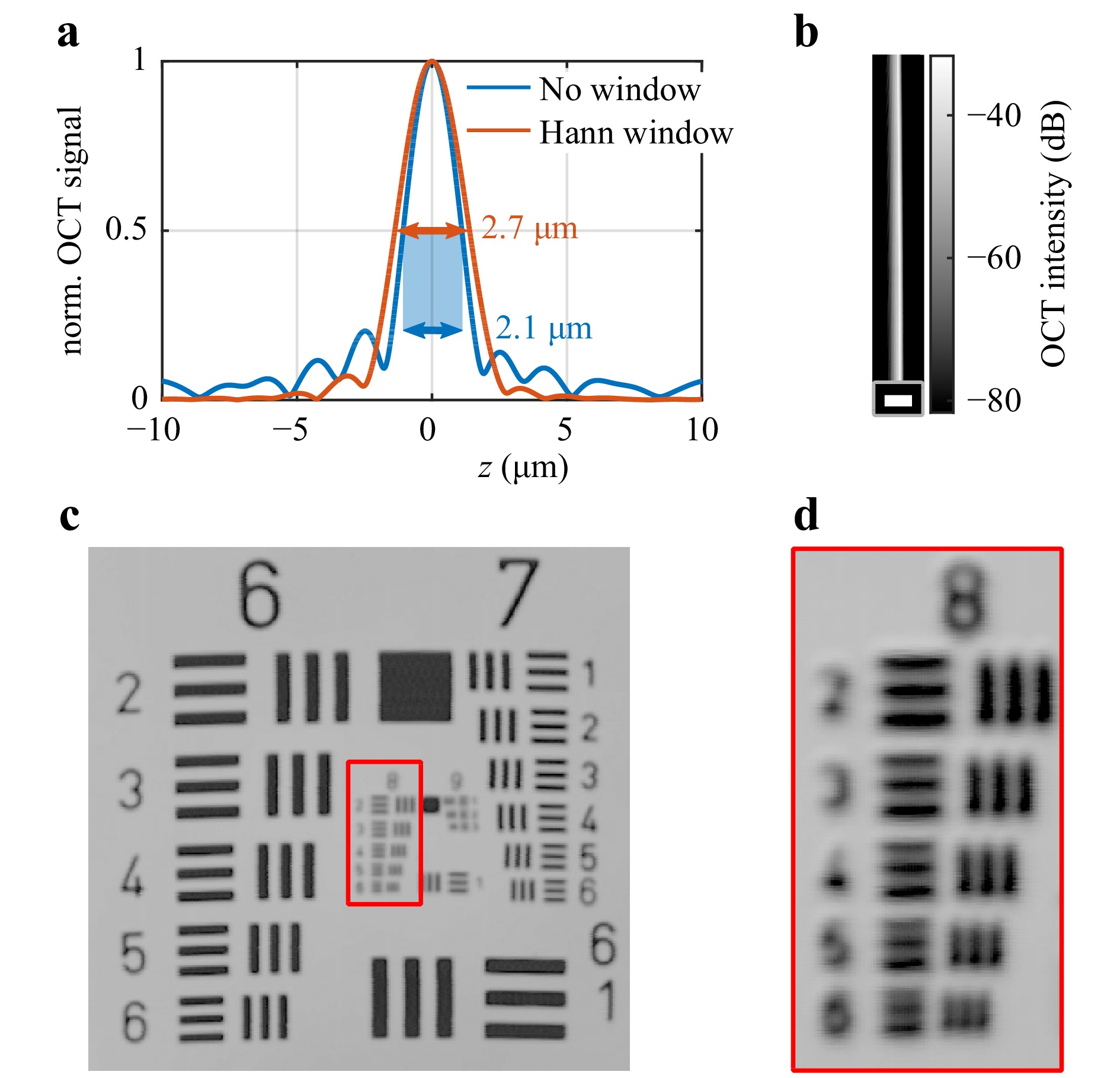
Fig. 2 Validation of the OCT system. a Two A-scans of the fused-silica substrate with applied Hann window (orange curve) and without window function (blue curve), measured in oil immersion. The full width at half maximum (FWHM) is 2.1 μm for the original measurement and 2.7 μm for the measurement with the applied Hann window. b Single B-scan of the substrate on a logarithmic scale. Throughout this paper, we normalize the OCT signal such that 0 dB corresponds to a 100% reflectivity. The scale bar is 20 μm. c OCT image of the USAF 1951 test target. d Resolved region of the target’s eighth group. The centre-to-centre spacing of the lines of the lowest element (group 8, element 6) is 2.2 μm (corresponding to 456.1 lp/mm).
A standard USAF 1951 test target immersed in immersion oil is used to characterise the lateral resolution of the OCT system. An OCT image of the test chart is presented in Fig. 2c. The elements of the eighth group can still be resolved, as shown in Fig. 2d, where the lowest element corresponds to a centre-to-centre line spacing of 456.1 lp/mm or 2.2 μm. Within the error bars, this measurement agrees with the lateral resolution obtained from Abbe’s diffraction limit of 1.9 μm.
In addition, we characterise the maximum sensitivity of our setup using the specular reflection of the interface between the immersion oil and the substrate, as described in Ref. 35 (see Methods section). We obtain a sensitivity
$ \mathrm{SNR}_\mathrm{max} $ of 105 dB, allowing for the detection of small refractive-index differences on the scale of$ \Delta n \approx $ 10−2 and below. -
Before examining 3D printed microstructures, we image a droplet of Nanoscribe IP-Dip photoresist on a planar substrate. Fig. 3a, b show 3D iso-surfaces of the OCT images, recorded on a sample with five-year-old photoresist and fresh photoresist, respectively. Notably, the aged photoresist shows a surprisingly large density of refractive-index inhomogeneities compared with the fresh photoresist. We interpret these “blobs” as being due to oligomer groups that have formed by thermal activation over time.
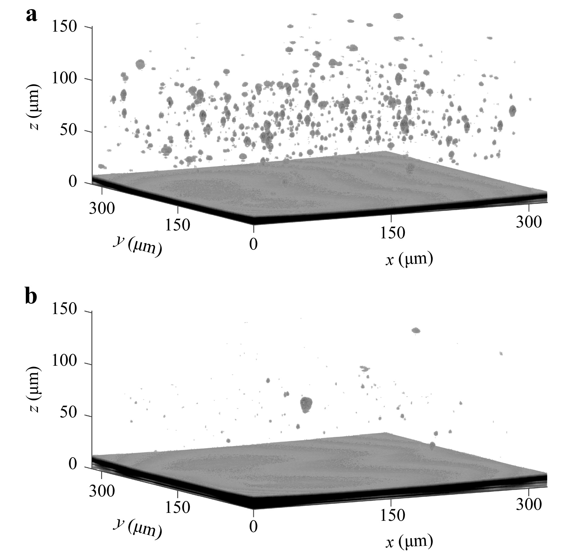
Fig. 3 Detection of refractive-index inhomogeneities in the volume of a photoresist (Nanoscribe IP-Dip). a five-year-old photoresist, b fresh photoresist. For both cases, we show the iso-surfaces of the OCT intensity at −65 dB.
To assess the influence of this number of scattering centres on multi-photon 3D laser printing, we perform calculations on the distortion of the laser printer’s writing focus, as depicted in Fig. 4 (see Methods section). For this purpose, we calculate the distribution of the scatterer diameters from Fig. 3a, assuming that the scatterers have a spherical shape. In the relevant OCT volume of 320 × 320 × 150 µm3 we observe a total of 761 scattering centres with diameters between 2.5 μm and 12.5 μm. For the focus distortion calculations, we take the average value of 6.5 μm as an exemplary particle diameter and calculate the total volume occupied by them in accordance with the total scattering volume obtained from the OCT measurements.
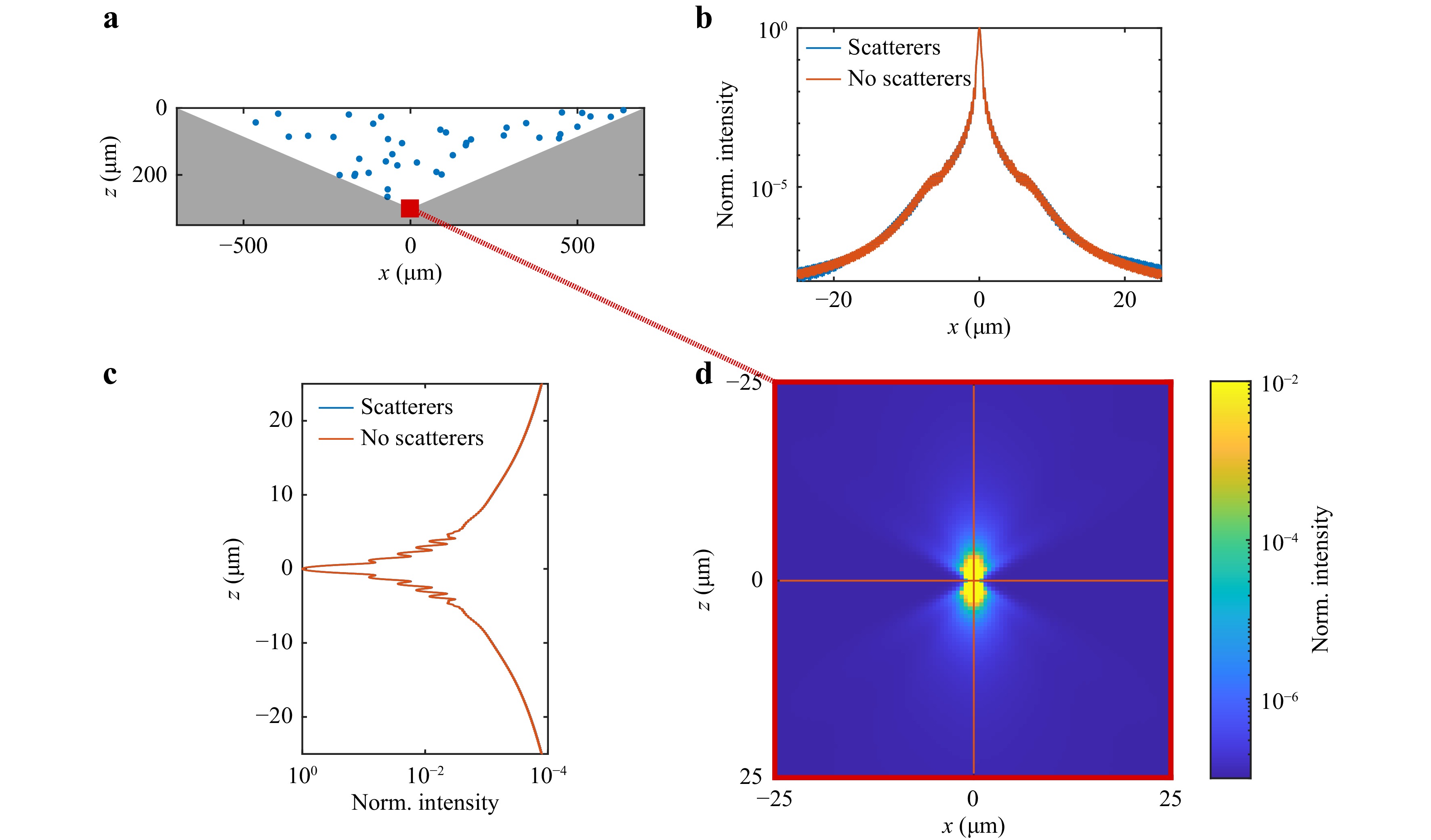
Fig. 4 Focus distortion simulations. a
$ xz $ -cut of the photoresist volume between objective lens and planar substrate used in our calculations. Randomly distributed scatterers with a diameter of 6.5 μm are shown as blue dots. The red square represents the laser focus. b Laser intensity distribution versus$ x $ -coordinate without (orange line) and in presence (blue line) of spherical scatterers. c Laser intensity versus axial$ z $ -coordinate. d Simulations of the resulting laser focus. The orange lines correspond to the cuts that were taken for the plots shown in panels b and c.A cross section of the simulated geometry is depicted in Fig. 4a. Scatterers (blue dots) are distributed randomly in the volume between the objective lens and the planar substrate. The simulation volume is a symmetric cone with a full opening angle of 133.6°, corresponding to an objective lens NA of 1.4. Furthermore, we assume that the observed inhomogeneities stem from small oligomer groups with a refractive index of
$ n_\mathrm{pol} \approx 1.545 $ in a medium with$n=1.51 $ . This corresponds to the refractive index measured for a photoresist polymerised using DLW. This value provides an upper bound for the oligomers.In Fig. 4a, the location of the focal spot is indicated by a red square. The
$ xz $ -cut of the intensity distribution is shown in Fig. 4d. The intensity distributions along the orange lines are shown in Fig. 4b ($ x $ -cut) and Fig. 4c ($ z $ -cut). From Fig. 4b, we see that the influence of the scatterers on the laser focus is small and becomes visible only at intensity levels in the range of 10−7 to 10−8 relative to the focus peak intensity. Hence, we conclude that their direct influence on the laser-writing process is presumably negligible. However, we foresee three indirect sources for unwanted printing imperfections. First, such inhomogeneities can serve as nuclei for micro-explosions that occasionally occur during multi-photon 3D laser printing36. Such micro-explosions may render the entire printed part useless. Second, these variations in the local cross-linking density before light exposure likely translate into variations in the local cross-linking density after printing. This means that printed parts that are intended to be homogeneous inside, are not actually mechanically, and/or optically homogeneous. The importance of this fact depends on the application. Third, these “blobs” may even remain on the surface of the printed parts if their cross-linking is sufficiently large to be not washed out by the developer. By using in-situ OCT, one can identify regions of inhomogeneous photoresist before the printing process and avoid the aforementioned problems. If necessary, “blobs” can likely be eliminated from the resist by filtering. -
Next, we examine the large planar surfaces of printed microstructures. As a test sample, we examine an array of cubes with a side length of 30 μm printed with a 63×/NA 1.4 objective lens onto a fused-silica substrate. To mimic an in-situ measurement, all samples are immediately imaged by OCT after printing without any additional steps in-between. A schematic of the sample geometry is shown in Fig. 5a. In this study, we measure the time-dependent OCT intensity of the planar interfaces at the bottom (polymer-substrate) and top (monomer-polymer) of a printed cube by averaging approximately 400 A-scans taken over the entire surface of the cube. Exemplary A-scan data are shown in Fig. 5b. The OCT intensity measured at the polymer-substrate interface (red squares) is stable over the entire measurement time of more than 16 hours (Fig. 5c). Hence, we conclude that our OCT setup is sufficiently stable over time. In sharp contrast, the OCT intensity measured at the monomer-polymer interface (green squares) exhibits very pronounced systematic variations, as shown in Fig. 5d. In the following, we present measurements of both of these interfaces consecutively.
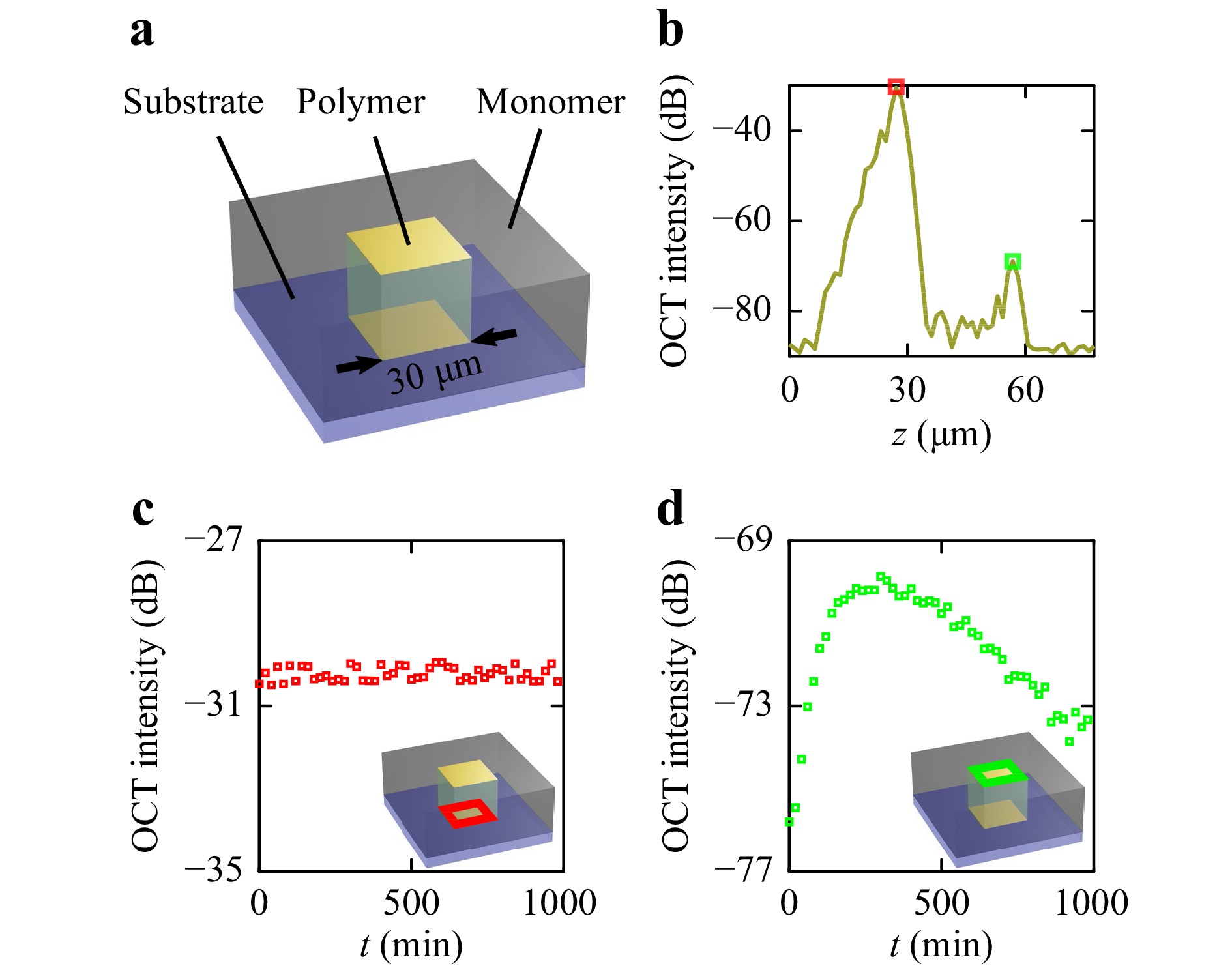
Fig. 5 Measurement of OCT intensity behaviour. a Scheme of the experiment. A printed polymer cube is immersed in a liquid photoresist (monomer) and is located on a fused-silica substrate. b Exemplary A-scan data of the printed cube. The left peak (red square) corresponds to the specular reflection of the substrate-polymer interface and the right peak indicates the monomer-polymer interface (green square). c Time-dependent OCT intensity of the substrate-polymer interface and d the monomer-polymer interface.
We start with the polymer-substrate interface. Because the refractive-index jump from polymer to fused silica can safely be assumed to be a jump on the scale of the wavelength of light, and because the refractive index of the fused-silica substrate is well-known (
$ n_\mathrm{sub} = 1.4525 $ at$ \lambda = 845 $ nm37), we can compare the measured OCT intensities to Fresnel’s equation in order to deduce the refractive index of the polymer. We use the interface between the monomer ($ n_\mathrm{mon} = 1.510 $ at$ \lambda = 845 $ nm38) and the substrate to calibrate the reflectivity of our setup. Refractive-index measurements of cubes (cf. Fig. 5) as a function of the writing power and writing velocity are shown in Fig. 6a. In this Figure, we plot the mean value of the polymer refractive index and its standard deviation based on the measurements of five nominally identical cubes for each value of the writing power and velocity. The laser power range is chosen between the polymerisation and overexposure thresholds at each velocity. The underlying calibration curve deduced from Fresnel’s equation is depicted in Fig. 6b, connecting the measured OCT intensity to the refractive index of the printed polymer (see Methods section). Clearly, this simple analysis based on Fresnel’s equation assumes flat interfaces and a discontinuous refractive-index jump. Furthermore, we will see that the refractive-index profile can generally be smeared out perpendicular to the interface and that the backscattering of light due to Bragg scattering can be important as well. These effects, as well as the effects of possible roughness within the interface plane, are neglected at this point.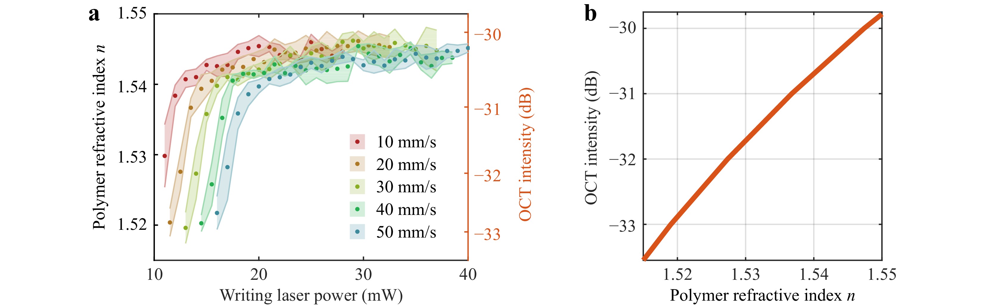
Fig. 6 Writing power dependence of polymerisation. a OCT intensity corresponding to the substrate-polymer interface (cf. Fig. 5) versus writing laser power. The OCT intensity on the right vertical scale is converted into the polymer refractive index on the left vertical scale. This conversion is based on the Fresnel reflection formulas for a polymer-substrate interface based on a refractive index of n = 1.4525 for the fused-silica substrate37 and of n = 1.510 for the unexposed photoresist38. The resulting calculated OCT intensity versus polymer refractive index is depicted in b.
Based on this simple analysis, we observe a monotonous increase in the deduced refractive index with increasing writing power. The observed saturation of the polymer refractive index in the range of
$ n = 1.545 $ is consistent with previous research on Nanoscribe IP-Dip structures by Dottermusch et al.39, in which the measurements were conducted using an ex-situ approach (i.e., in air). Furthermore, the obtained dependencies can be considered from the viewpoint of the degree of conversion (DC) because the refractive index of the polymer directly depends on the DC value40. It has been shown that there is a saturation in DC for Nanoscribe IP-Dip printed structures regardless of the printing speed, which is consistent with our measurements41. In summary, in-situ OCT combined with DLW can potentially facilitate the printing of microstructures with more than two tailored refractive indices42 (provided there are still clear refractive-index discontinuities), as it is proving to be a sensitive and fast method for extracting the refractive index of a printed material. Along these lines, it should be possible to optimise the printing parameters on-the-fly, such that the desired refractive index of the printed material can be realised quickly.Next, we investigate the origin of the time-dependent OCT intensity of the monomer-polymer interface for the cubes printed with different writing laser powers at a scanning speed of 30 mm·s−1. Fig. 7 depicts the OCT intensity versus time (blue curves) arranged in a 6 × 3 matrix. Each row consists of cubes printed with a fixed writing laser power. The columns in the matrix refer to the three configurations. The first column corresponds to cubes measured immediately after printing (undeveloped case). The second and third columns contain measurements of printed structures that are further developed in the indicated solvent (acetone and propylene glycol methyl ether acetate, PGMEA, respectively), followed by re-immersion in the same photoresist. As a control experiment, we also measure and plot the (stable-in-time) OCT intensity of the polymer-substrate interface for each cube (dashed orange curves).
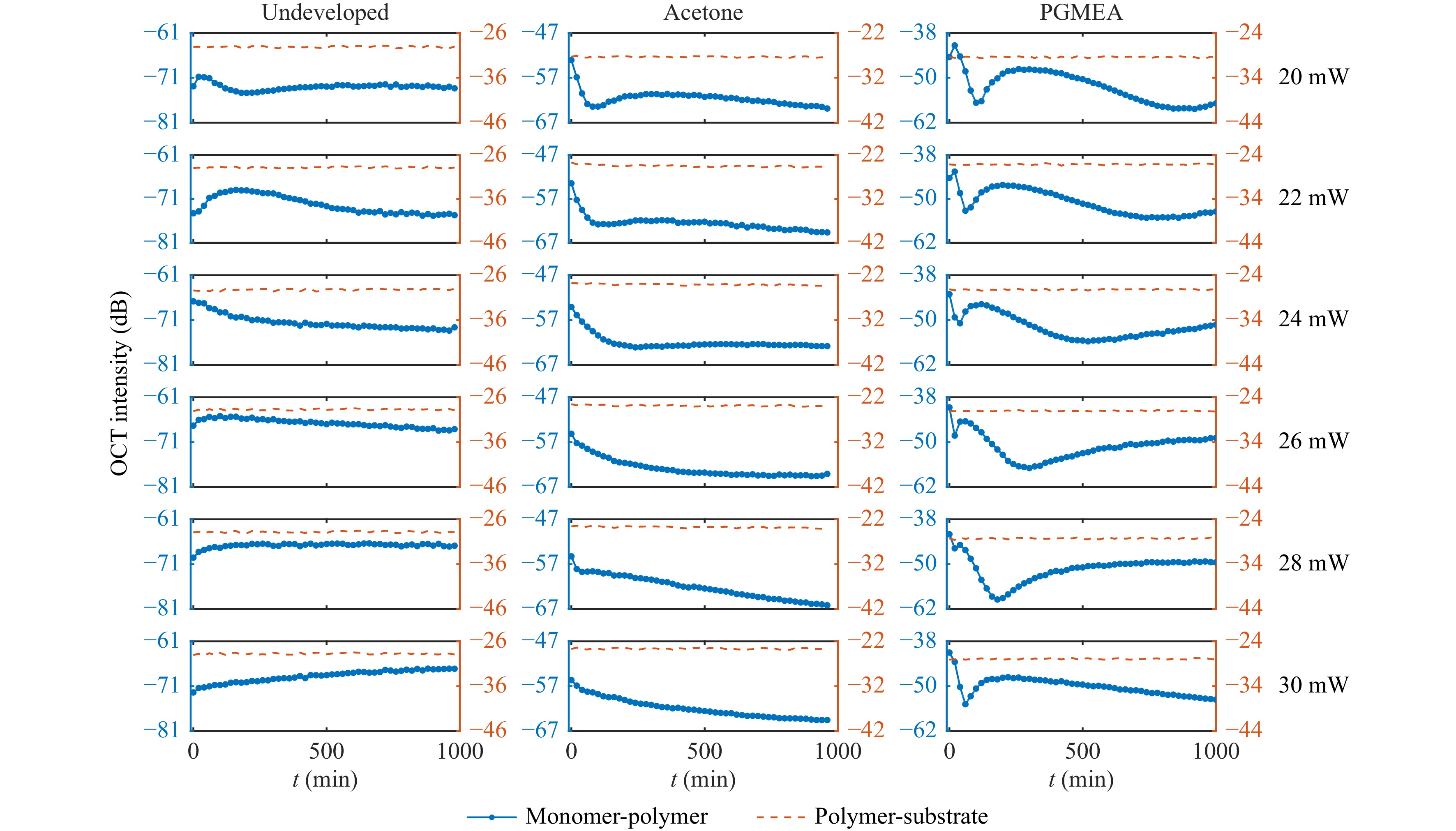
Fig. 7 Time-dependent OCT intensity. OCT intensity (blue curves) corresponds to the polymer-monomer interface (cf. Fig. 5). As a control experiment, we also measure the OCT intensity which corresponds to the polymer-substrate interface (dashed orange curves). The shown panels form a 6 × 3 matrix. Within each row of this matrix, a fixed laser power is used for the printing of the cube, as indicated on the right-hand side. The three columns of this matrix refer to different conditions. In the first column, labelled “undeveloped”, the cube is exposed to the writing laser; this step is immediately followed by OCT imaging. In the second and the third column, exposure to the writing laser is followed by washing in acetone and PGMEA, respectively. These samples are imaged by OCT after re-immersion in the same photoresist (Nanoscribe IP-Dip).
Notably, the time dependence of the OCT intensity is completely different between all three cases. For the undeveloped sample, no correlations between the writing laser power and the OCT intensity curve shape are observed. The curves in this case can exhibit oscillatory behaviour (20 and 22 mW), have a downward or upward trend (24, 26 and 28 mW), or even increase linearly (30 mW). In sharp contrast, the acetone-developed structures show an exponential-like decay with a tendency for a decreasing decay constant with an increasing laser power (curve flattening). Finally, PGMEA-developed cubes show pronounced oscillations, the extrema of which appear earlier in time with increasing laser power.
Conceptually, the measured OCT intensity variations correspond to variations in the intensity reflectivity of the polymer-monomer interface. If the spatial refractive index profile
$ n(z) $ at this interface is a simple step function, the resulting reflectivity can be calculated using Fresnel’s equations. However, in reality, this refractive-index transition might not be a sharp step function, but rather a continuous transition with a finite width extending over a significant fraction of the wavelength, yielding invalid Fresnel equations in their usual form. To further evaluate this aspect, we perform model calculations using the transfer-matrix method for extracting the intensity of the reflectivity$ R $ for different assumed spatial behaviours of the refractive index at the polymer-monomer interface. Exemplary spatial refractive-index profiles are shown in Fig. 8a. For simplicity, we model these profiles$ n(z) $ using two parameters: a transition width$ w $ and an exponential parameter$ e $ , which smoothes out the transition profile$ n(z) $ proportional to$ \pm z^e $ (see Methods section). In all calculations, the lower and upper refractive indices$ n_0 = 1.51 $ and$ n_1 = 1.545 $ (corresponding to unpolymerised liquid and polymerised solid photoresist, respectively) are kept the same.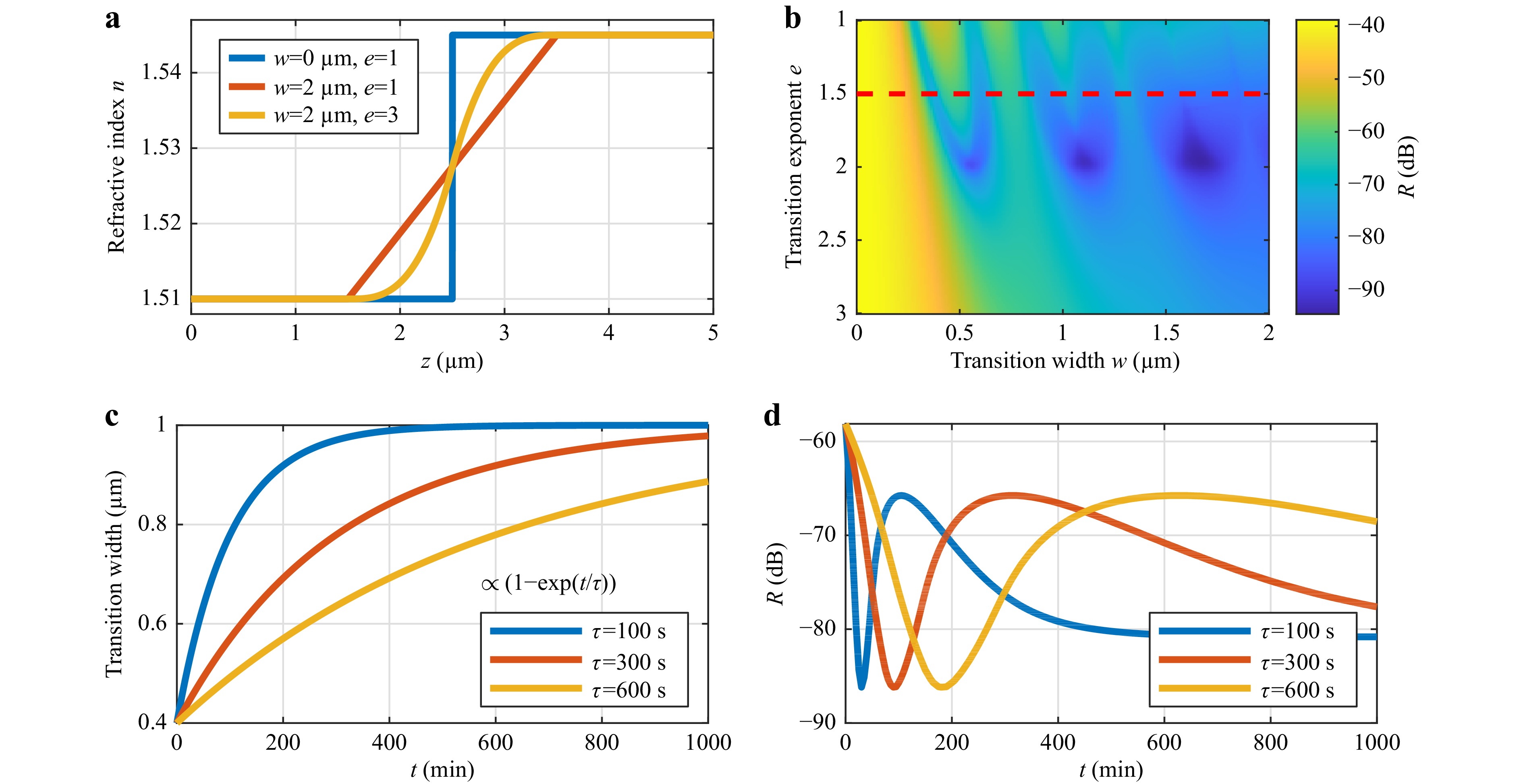
Fig. 8 Transfer-matrix-based reflectivity calculations of the monomer-polymer “interface”. a The refractive-index transition profile is modelled using two parameters: a transition width
$ w $ and a transition exponent$ e $ (see main text). b Reflectivity versus$ w $ and$ e $ , calculated (by averaging) for a box-shaped intensity profile with a spectral width of$ \Delta\lambda = 135 $ nm centred around the$ \lambda_0 = 845 $ nm wavelength. c Exemplary assumed functions for the temporal behaviour of the transition width$ w(t) $ . d Behaviour of reflectivity versus time, obtained by resampling the reflectivity data$ R(w,e) $ for$ e = 1.5 $ from panel b using the function$ w(t) $ plotted in panel c. The obtained reflectivity$ R $ oscillates versus time. This behaviour can be compared to the experimentally measured traces plotted in Fig. 7. For example,$ R = -80 $ dB equals a reflectivity of$ R = 10^{-8} $ and an OCT intensity of$ -80 $ dB (cf. Fig. 7).In Fig. 8b, we plot the obtained reflectivity with respect to
$ w $ and$ e $ . In these calculations, we mimic a broadband light source with a central wavelength of$ \lambda_0 = 845 $ nm and a spectral width of$ \Delta\lambda = 135 $ nm by averaging the reflectivity values obtained from monochromatic calculations over different wavelengths. Notably, for a smaller$ e $ , the reflectivity$ R $ oscillates with an increasing width$ w $ . By contrast, for$ e\gtrapprox2.5 $ ,$ R $ decreases monotonously with increasing$ w $ . Hence, we conclude that the reflectivity obtained from a graded-index step depends critically on both, the width of the “step” as well as on its exact shape.For a better comparison with the experimental time-dependent measurement data (Fig. 7), we resample the calculated width-dependent reflectivity data to the time axis. For this purpose, we assume that the transition width increases exponentially from 0.4 μm to 1 μm, as indicated in Fig. 8c. With respect to the experiment, this behaviour could be explained by a swelling of the polymer network during the development step in a solvent (in PGMEA or acetone), followed by the out-diffusion of the solvent after re-immersion into the photoresist. Finally, by resampling
$ R $ to time$ t $ using the curves from Fig. 8c, we obtain time traces in Fig.8d that are similar to the time-dependent OCT intensity measured after development in PGMEA (Fig. 7). It is desirable to refine these simulations in order to better reproduce the experimentally measured curves. However, because the precise behaviour of the refractive index of the polymer-monomer interface is not known and has to be assumed, this goal currently appears out of reach. In other words, there are too many free parameters for the given measured data to obtain a unique reconstruction.We note in passing that the undeveloped cubes are essentially not visible in OCT (not depicted) if we use the 25×/NA 0.8 objective lens for printing, instead of the 63×/NA 1.4 lens. The same effect is observed for both IP-Dip and IP-S (Nanoscribe) photoresist. We interpret this finding as the refractive-index profile for a lower magnification being more smeared out in space, resulting in a much lower reflection from the transition region between polymer and monomer.
The final step in the study of planar interfaces is an evaluation of the thickness of the printed plates located on polymer supports. A set of plate samples in the form of a square cuboid with a base length of
$ 30 $ μm and varying height is fabricated by DLW and immediately measured by OCT.Each A-scan is converted to intensity units and fitted by the sum of the two Gaussians. These two Gaussians represent the top and bottom planar polymer-monomer interfaces. Thus, the distance between the two fits corresponds to the plate thickness. Finally, we average the thickness over the entire plate surface to obtain the mean thickness value and its standard deviation. Fig. 9 demonstrates a comparison of plate thickness values taken from OCT versus the ones measured by SEM, as well as an exemplary SEM image of a plate sample and A-scan data. Based on a comparison of SEM- and OCT-measured plate thicknesses, we conclude that one can in situ determine the thickness of polymer planar structures with sufficient accuracy. The minimum resolved plate has a thickness of 3.1 μm, which is close to the FWHM of the point spread function (2.7 μm, cf. Fig. 2a). The evaluation of thinner plates is problematic because plate bending occurs at lower thicknesses.
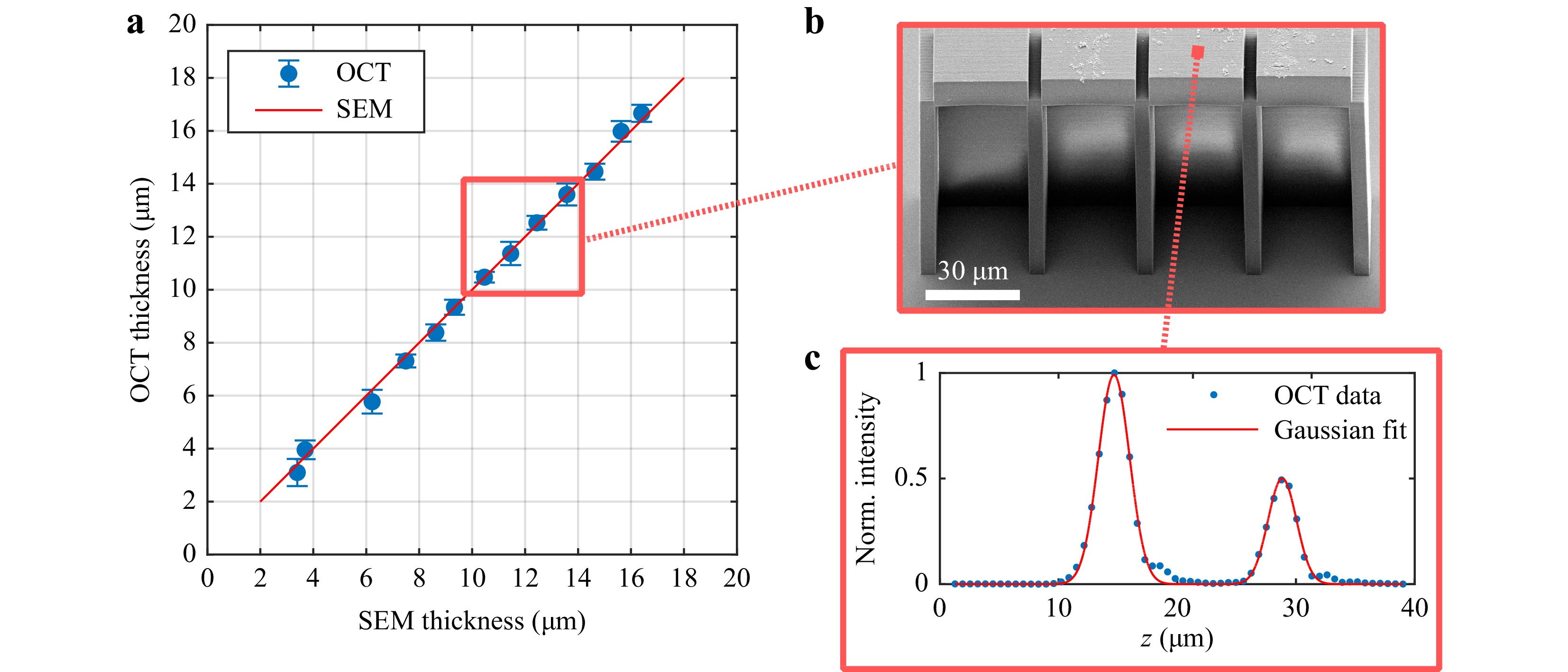
Fig. 9 Evaluation of polymer plate thickness. a Comparison of thickness values obtained from SEM and OCT measurements. b Exemplary oblique-view (45 degrees) SEM image of one of the samples used for the analysis shown in panel a. c Exemplary A-scan data (blue dots) taken from the plate part (cf. panel b). The red curve corresponds to a fit using the sum of two Gaussian functions. The OCT thickness shown in panel a is defined as the distance between the peaks of the two Gaussians.
-
To examine the OCT signal of the complex interfaces, we print a series of 3D microstructures. First, we fabricate a 3D test sample in the form of a half-sphere with a radius of 50 μm (Fig. 10a). The OCT image of the printed half-sphere consists of a bright reflective spot in the centre of the structure and a weak scattering signal around it. For better visualisation, we plot the maximum OCT intensity of the half-sphere projected onto the
$ xy $ -plane using a false colour scale (Fig. 10b). The spot stems from the specular reflection of rays incident at an angle corresponding to$ \mathrm{NA}_\mathrm{eff} = 0.22 $ . We calculate the relevant spot perimeter that it would occupy on the half-sphere and depict it as a black solid circle in Fig. 10b. Clearly, the observed specular reflection area (yellow region) coincides with the calculated perimeter. Hence, this experiment validates the value of the effective numerical aperture of our OCT system.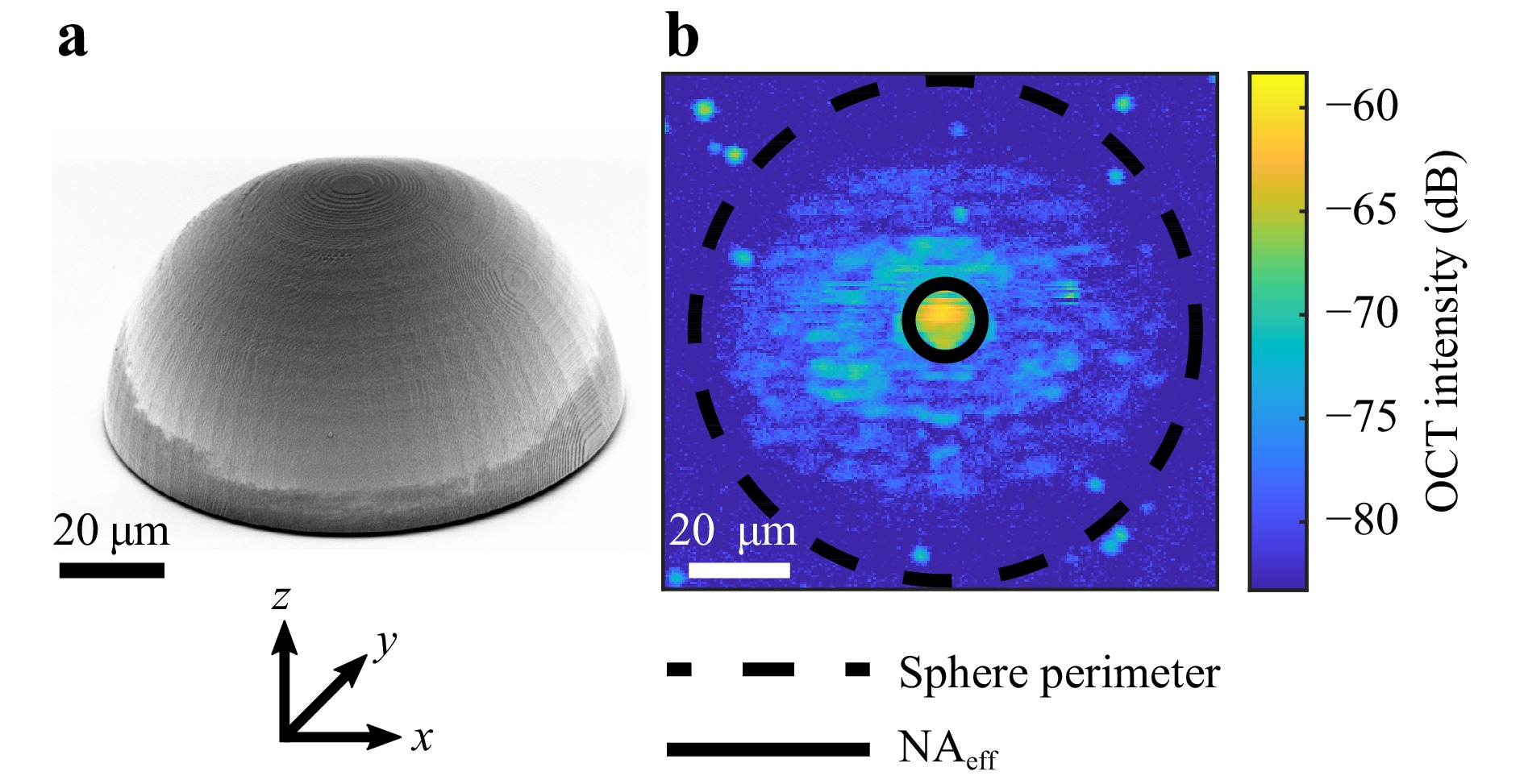
Fig. 10 Images of a printed half-sphere. a SEM image of a printed half-sphere. b Maximum OCT intensity projected onto the
$ xy $ -plane using a false-colour scale. The black dashed circle corresponds to the perimeter of the sphere. The black solid circle corresponds to the effective numerical aperture$ \mathrm{NA}_\mathrm{eff} = 0.22 $ of the OCT apparatus.Next, we print two identical cubes with side lengths of 50 μm using different printing configurations (Fig. 11a). The cube on the left-hand-side is fabricated using cross-directional hatching, i.e., the hatching direction changes with each slicing layer by 90°. The cube on the right-hand-side is printed with uni-directional hatching, i.e., the hatching direction remains constant. Both cubes have slicing and hatching distances of 200 nm. Although there are no apparent differences between the two cubes in the SEM image, we observe significant differences in their 3D OCT reconstructions, which are shown in Fig. 11b. For the cross-hatched cube, the OCT contrast can be retrieved not only for the planar reflective polymer-monomer surface but also for all vertical sidewalls. This observation indicates that cross-hatching results in a non-uniform distribution of the refractive index between the slicing layers. This nonuniformity allows for the detection of the backscattered signal from surfaces that are not perpendicular to the optical axis. In Fig. 11b, the OCT signal from the interior of the cube is much smaller than that from the surfaces. Hence, the OCT representation of the cube is a hollow cube (not depicted).
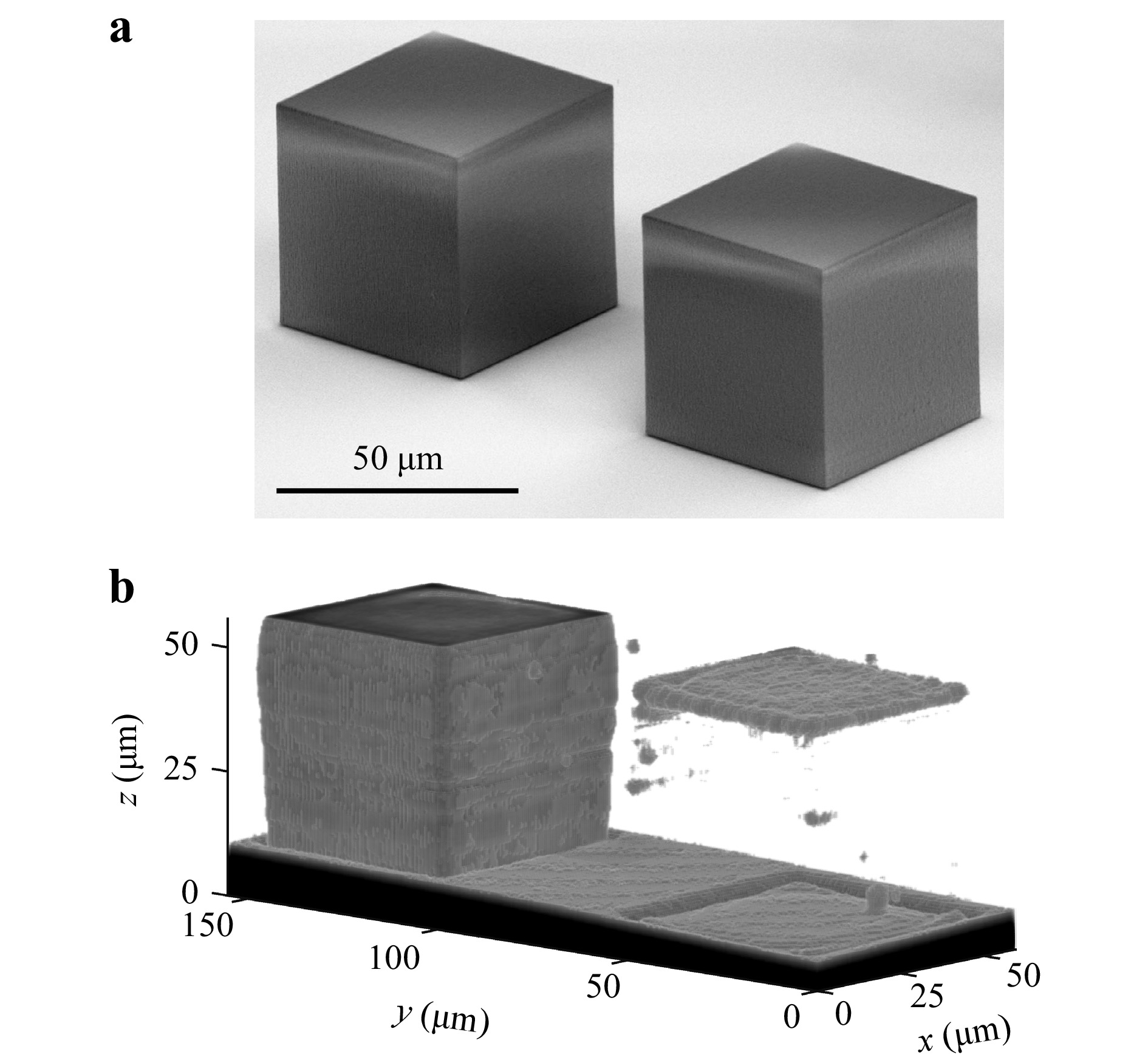
Fig. 11 Images of cubes. a SEM image of two printed cubes. The left cube is printed using cross-directional hatching, the right cube using uni-directional hatching (see main text). b 3D OCT reconstructions (iso-surfaces at −73 dB OCT intensity) of the two cubes. Clearly, the vertical sidewalls are only visible for the left cube.
To further investigate this aspect of light scattering (rather than specular reflection), we print an array of cross-hatched prisms with various slicing distances (from 140 to 300 nm in steps of 10 nm) and printing laser powers (from 18 to 28 mW in steps of 1 mW). The hatching distance is 200 nm for all structures. The geometry of a prism is chosen because none of the surfaces of a prism leads to specular reflection along the optical axis. Therefore, the OCT signals of such structures are exclusively due to light scattering. To allow for a direct comparison, the SEM images and resulting 3D OCT reconstructions of the prisms are shown in Fig. 12. This Figure shows that the OCT intensity of the prism samples does not only depend on the writing laser power, but also on the slicing distance. Prisms with slicing distances of 200, 260, and 280 nm are completely reconstructed using OCT. A difference as small as 20 nm can completely change the backscattering signal and cause the OCT intensity of the prism to be below the chosen threshold value. The prisms are also partially recognisable at a slicing value of 140 nm. These experimental findings clearly indicate that the light scattering from the interior of these prisms depends on the chosen slicing distance. We interpret these findings in that the slicing procedure leaves behind small refractive-index variations in the volume of the printed specimen. The amplitude of these variations depends on the printing parameters and the photoresist used, and especially on the size of its proximity effect. These refractive-index variations lead to the backscattering of light. Considering the sizes involved, Rayleigh scattering43 is expected to play a minor role, leaving Mie scattering and Bragg scattering as possible candidates. Owing to the periodicity of the slicing distances, Bragg backscattering is the most likely candidate. For Bragg backscattering, the period of modulation must be equal to half the wavelength of the light within the photoresist. This period is equal to 280 nm for the central wavelength of the SLD and accurately matches the slicing value, showing the best OCT contrast (highlighted in red). This Bragg scattering from refractive-index inhomogeneities (originating, for example, from cross-hatching) also explains the sensitivity of the OCT signal to the value chosen for the other slicing distances in Fig. 12 (see Supplementary Information and Figure S2). From the OCT signal observed for IP-Dip, we estimate the amplitude of the periodic refractive-index modulation to be of the order of
$ \Delta n \approx 10^{-3} $ .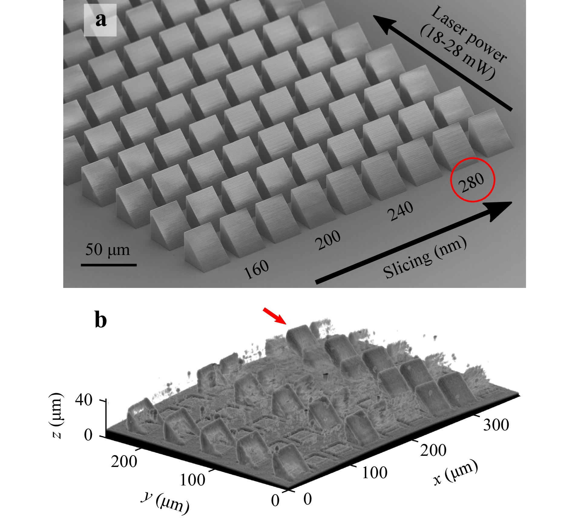
Fig. 12 Images of prisms. a SEM image of an array of printed polymer prisms. We use cross-hatching with the indicated slicing distances for the printing process. The slicing distance that corresponds to the central Bragg wavelength is highlighted by a red circle. In addition, we vary printing laser power along the orthogonal direction in steps of
$ 1 \text{ mW} $ between adjacent rows. b OCT reconstructions (iso-surfaces at −64 dB OCT intensity) of the same sample. Note that the visibility of the sidewalls depends on the slicing distances in a complex manner due to Bragg backscattering of the light.In any case, when looking at the results shown in Fig. 12 in the spirit of using OCT as an in-situ diagnostic tool during the printing process of, for example, micro-optical components such as lenses, one should ideally neither see any of the surfaces not perpendicular to the optical axis nor should one measure an OCT signal from the interior. The fact that one sees other surfaces indicates optical imperfections in the printed specimens. These imperfections may deteriorate the performance of the printed device, depending on the application.
Finally, we fabricate and visualise two more complex 3D microstructures: a buckyball and “benchy”, a small boat that is frequently used as a benchmark in different 3D additive manufacturing approaches. In this case, we implement cross-hatching and slicing/hatching distances of 200 nm to achieve a high OCT contrast owing to the above-described effect of Bragg scattering, which is perhaps the polar opposite of the best sample quality. Fig. 13 shows SEM images and 3D OCT reconstructions that can be compared directly.
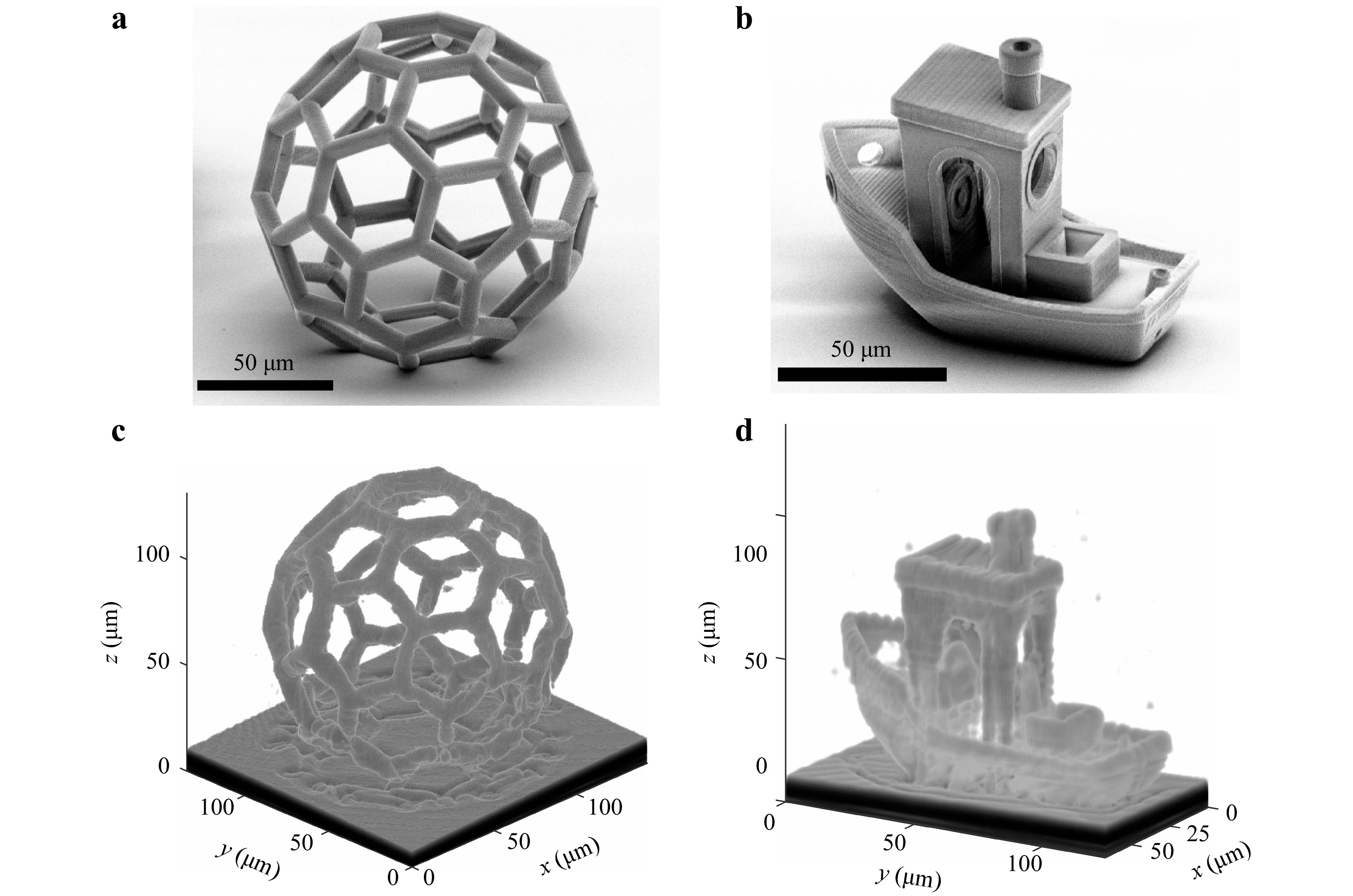
Fig. 13 Images of a buckyball and a “benchy” boat. a and b SEM images. For the printing process, we used cross-hatching with a hatching/slicing distance of 200 nm and a laser-focus speed of 2 cm·s−1. c and d OCT reconstructions (iso-surfaces at −71 dB and −53 dB OCT intensity, respectively) of the same samples.
-
In summary, we have demonstrated the possibility of using Fourier-domain OCT as a fast in-situ diagnostic tool for multi-photon 3D laser printing. The key performance parameters of our OCT system are as follows: 1.9 μm lateral resolution, 2.7 μm axial FWHM (which is expected to be comparable to the axial resolution), up to 1 mm axial field-of-view for one A-scan, 40 μs acquisition time for one A-scan (equivalent to a frame rate of 25 kHz), and 105 dB sensitivity or signal-to-noise ratio for a single experiment. These numbers can be compared to those of state-of-the-art OCT systems used for other purposes, e.g., in Ref. 44, 45. By “fast”, we mean that the OCT data acquisition time for a complete 3D data set of a certain volume is more than two orders of magnitude smaller than the typical printing time for the same volume. Therefore, one could add a couple of inspections during a print job without significantly increasing the overall print time. Importantly, if conducted properly, the OCT process does not lead to unwanted polymerisation, even when used extensively. Our home-built OCT apparatus operates under real-life operating conditions, allowing us to readily integrate it into existing 3D laser printers. Moreover, we have shown a wide range of applications for this OCT instrument. This includes photoresist-homogeneity inspection before printing, in-situ evaluation of the laser-power-dependent refractive index of polymerised regions, time-dependent diffusion processes at the monomer-polymer interfaces over timescales on the order of hours, thickness measurements of printed parts, surface roughness and volume-homogeneity inspection of printed parts by backscattering of light, and perhaps most obviously, 3D reconstructions of printed microstructures that can be compared with the targeted 3D computer model.
The OCT approach is also expected to work if the excitation process in 3D laser printing, which involves two-photon absorption, is replaced by a two-step absorption process14, provided the OCT spectrum does not overlap with the two-step excitation wavelength.
-
Sensitivity characterization To calculate the signal-to-noise ratio (SNR) of the OCT setup, we use the method of specular surface reflection described in Ref. 35 with a fused silica substrate as a specular reflector and immersion oil as a medium. SNR is calculated as follows:
$$ \mathrm{SNR}_{\mathrm{max}} (\mathrm{dB}) = 20\,\mathrm{log}\left(\dfrac{I_{\mathrm{sub}}}{\sigma_{\mathrm{bg}}}\right)-10\,\mathrm{log}(R_{\mathrm{sub}}) $$ (1) where
$ I_\mathrm{sub} $ is the OCT intensity of the oil-substrate interface,$ \sigma_{\mathrm{bg}} $ is the standard deviation of the background intensity away from the substrate, and$ R_{\mathrm{sub}} $ is the Fresnel intensity reflection coefficient of the oil-substrate interface. The known refractive index of the glass substrate of$ 1.4525 $ and that of the used immersion oil of$ 1.510 $ lead to$ R_{\mathrm{sub}} = 3.77\times10^{-4} $ , which is equivalent to an OCT intensity of$ -34.24 $ dB. The sensitivity$ \mathrm{SNR}_{\mathrm{max}} $ of$ 105 $ dB quoted in the main text refers to a frame rate of$ 25 $ kHz and a single measurement. Averaging further improves this value.Multi-photon 3D laser printing Laser printing is performed using a commercially available DLW apparatus Nanoscribe Professional GT with a
$ 63\times $ /NA$ 1.4 $ objective lens in the dip-in mode. All samples are printed using IP-Dip (Nanoscribe) photoresist. In addition, we print cube samples in IP-Dip and IP-S (Nanoscribe) photoresists using a$ 25\times $ /NA$ 0.8 $ objective lens. For a two-photon absorption and an ideal photoresist, the resolution of the printing process can be estimated from the full width at half maximum (FWHM) of the squared focus intensity profile along the lateral (and axial) directions. For the$ 25\times $ objective lens, we obtain$ 400 $ nm (and$ 2300 $ nm) for the$ 63\times $ objective lens$ 250 $ nm (and$ 600 $ nm).OCT measurements The printed samples are measured on the OCT setup immediately after printing unless stated otherwise. We perform OCT measurements in the same photoresist used for laser printing as an immersion medium. To eliminate undesired air-glass specular reflections, we add a drop of immersion oil on top of the substrate. For all experiments reported herein, the power from the superluminescent diode, measured at the entrance pupil of the microscope objective lens, is approximately
$ 4.1 $ mW). The$ 1/e^2 $ intensity diameter of the OCT beam at the same point is$ 1.2 $ mm). Assuming a$ 70\% $ optical intensity transmission of the microscope lens, we estimate the light intensity in the focal plane to be$ 60 $ kW/cm2. This intensity level do not lead to a polymerisation of previously unpolymerised parts in our experiments. To convert the OCT data into an absolute z axis, one needs to make an assumption regarding the group index. Because the materials involved in our work are only weakly dispersive, we assume that the group index is equal to the refractive index at the centre wavelength of the OCT superluminescent diode. For the unpolymerised monomer, we use$ n_{\mathrm{mon}} = 1.51 $ ; for the polymer, we use$ n_{\mathrm{pol}} = 1.545 $ .Focus distortion calculations To calculate the possible influence of the detected refractive index inhomogeneities on the focus, we describe the system as follows: the illumination is approximated by a monochromatic circularly polarized plane wave with a wavelength of
$ 790 $ nm. This wave is refracted into the photoresist containing the described scatterers by an objective lens with a numerical aperture of$ 1.4 $ and a focal length of$ 4.125 $ μm.Simulating the focal spot, including the perturbations induced by the scatterers, is a computational challenge for many numerical methods owing to the large volume of computational domain needed. The relevant domain is the cone-shaped volume between the lens and the focal spot. Therefore, we simulate the scattering using the T-matrix method46, in which simulations are limited not by the total size of the volume, but by the size and number of the individual scatterers. To include focusing by the objective lens into the simulations, we use the method of47 before the T-matrix calculations. Therefore, the simulation can be summarised as a three-step process. First, the angular spectrum representation of the focused light behind the lens is calculated. This field is the background field for the following scattering calculations. Second, a random arrangement of scatterers is generated in a cone shaped volume and, finally, the scattered field is calculated.
Details of the calculation of the focal field can be found in the Ref. 47. In short, the electric field of the incoming beam is refracted at the lens onto a spherical sector centred at the focal spot. The radius and opening angle of the spherical sector are determined by the focal length and numerical aperture of the lens. The refracted field is then converted to an angular spectrum representation of the field in the focal plane. The angular spectrum representation can be propagated to an arbitrary point within the resist by applying suitable phase factors. Thus, we obtain the background field at the position of each scatterer.
After obtaining the background field, the next step is to generate a random arrangement of refractive index inhomogeneities. For this, we generate random positions within the cone between the lens and the focal spot. Random positions are only added to a simulated sample if a newly added scatterer does not overlap with existing scatterers. To improve the efficiency of the subsequent T-matrix calculation, the scatterers are approximated by spheres of a fixed diameter. We deduced the diameter and volume distribution of the scatterers from the OCT measurements, as described in the main text.
The T-matrix of spherical scatterers can be calculated analytically48. Typically, the next step is to calculate the interactions between particles. However, owing to the high number of particles, multi-scattering processes are extremely resource-demanding in computational terms. Therefore, we approximate the total scattering by neglecting this interaction. We evaluate the scattered field around the focal spot for each scatterer. Finally, we consider the coherent sum of the individual scattering of each particle.
Refractive-index calculations We treat the polymer-substrate interface signal in terms of the Fresnel reflectivity, taking the monomer-substrate interface signal as the reference value for the recalculation from the OCT intensity to the Fresnel coefficient. We extract the refractive index of the polymer from the OCT data according to the following equation:
$$ n_\mathrm{pol} = n_\mathrm{sub}\dfrac{1+\sqrt{\dfrac{\mathrm{FT}_\mathrm{pol-sub}^2}{k}}}{1-\sqrt{\dfrac{\mathrm{FT}_\mathrm{pol-sub}^2}{k}}} $$ (2) $$ k = \mathrm{FT_{mon-sub}^2}\left(\dfrac{n_\mathrm{mon}+n_\mathrm{sub}}{n_\mathrm{mon}-n_\mathrm{sub}}\right)^2 $$ (3) where
$ n_\mathrm{pol} $ ,$ n_\mathrm{mon} $ ,$ n_\mathrm{sub} $ are the refractive indices of the polymer, monomer, and substrate, respectively,$ \mathrm{FT}_\mathrm{pol-sub} $ and$ \mathrm{FT}_\mathrm{mon-sub} $ are the Fourier-transform OCT signals of the polymer-substrate and monomer-substrate interfaces, respectively. The resulting calibration curve for the recalculation of the measured OCT intensity with respect to the polymer refractive index is shown in Fig. 6b.Transfer-matrix calculations For the transfer-matrix calculations, we use code written by Shawn Divitt, which is available in the Matlab File Exchange49. In particular, we use a simulation range of
$ 5 $ μm, which we discretize into layers with a thickness of$ 2 $ nm. The refractive-index step, which is centred around$ x_0 = 2.5 $ μm, is implemented by$$ n(x) = \begin{cases} n_0 & \text{for } x < x_0-\frac{w}{2} \\ n_0 + \frac{n_1-n_0}{2} \times \left| \frac{x-(x_0-w/2)}{w/2} \right|^h & \text{for } x_0-\frac{w}{2} < x < x_0 \\ n_1 - \frac{n_1-n_0}{2} \times \left| \frac{x-(x_0+w/2)}{w/2} \right|^h & \text{for } x_0 < x < x_0+\frac{w}{2} \\ n_1 & \text{for } x > x_0+\frac{w}{2} \\ \end{cases} $$ (4) Herein, we assume real refractive indices
$ n_1 = 1.51 $ and$ n_2 = 1.545 $ with no losses. Calculations are performed for perpendicular incidence. To account for the broadband light source in the OCT, we perform calculations for different wavelengths centred around$ \lambda_0 = 845 $ nm in the range of$ 135 $ nm and in steps of$ 5 $ nm. The final$ R $ is obtained by averaging. -
This work was funded by the Deutsche Forschungsgemeinschaft (DFG, German Research Foundation) under Germany’s Excellence Strategy 2082/1-390761711 (Excellence Cluster “3D Matter Made to Order”). The authors acknowledge support from the Helmholtz program Science and Technology of Nanosystems (STN), Karlsruhe School of Optics and Photonics (KSOP), and Carl Zeiss Foundation. The authors are grateful to Tilman Schmoll (Carl Zeiss) for his valuable advice on establishing the OCT setup and Antonia Lichtenegger (Medical University of Vienna) for her help during the preparation of this study. We would also like to thank Richard Wagner (KIT) for his help with the numerical focus calculations.


 DownLoad: